Lecture 19: PID Design with the Root Locus and Python
This lecture brings the previous ones together in a complete design. We meet transient specifications with PD compensation (Lecture 17) and a steady-state specification with PI compensation (Lectures 12 and 18). The work is carried out first analytically, on the root locus, and then computationally in Python, so that each approach can check the other.
The problem
The plant is stable and third order:
$$G(s) = \frac{s+8}{(s+3)(s+6)(s+10)}.$$We want a unity-feedback controller that achieves:
- a percentage overshoot of at most $20\%$;
- a peak time equal to $\tfrac23$ of the uncompensated (P-only) peak time $T_{p,u}$;
- zero steady-state error to a step.
The plan. A PID controller can be written as a PD part times a PI part:
$$C(s) = K\,(s + z_D)\,\frac{s + z_I}{s}.$$This factorization separates the tasks. Step 1 designs the PD part for the transient (specifications 1 and 2). Step 2 adds the PI part for the steady state (specification 3). The design assumes that one pair of second-order poles dominates the closed loop, in the sense of Lecture 8.
Step 1: the transient
The uncompensated design. From Lecture 7, $20\%$ overshoot corresponds to
$$\zeta = \frac{-\ln 0.2}{\sqrt{\pi^2 + \ln^2 0.2}} = 0.456.$$The root locus of $KG$ has poles at $-3$, $-6$, $-10$, a zero at $-8$ and asymptotes at $\pm90^\circ$. The $\zeta = 0.456$ line meets the dominant branches at
$$s = -5.415 \pm j10.57,\qquad K \approx 121.5,\qquad T_{p,u} = \frac{\pi}{\omega_d} = \frac{\pi}{10.57} = 0.297\ \text{s}.$$The target pole. The required peak time is $T_p = \tfrac23(0.297) = 0.198$ s. Keeping the same $\zeta$ (to keep the overshoot) and working backwards through the formulas of Lecture 7:
$$\omega_d = \frac{\pi}{0.198} = 15.86,\quad \omega_n = \frac{\omega_d}{\sqrt{1-\zeta^2}} = 17.82,\quad \zeta\omega_n = 8.13\;\Longrightarrow\; s_d = -8.13 + j15.86.$$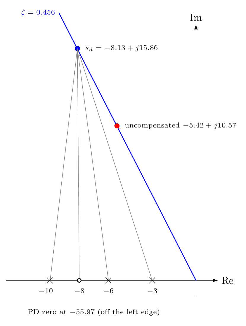
The PD zero. As in Lecture 17, we place the zero so that $s_d$ satisfies the angle condition. With $\theta$ the angles of the vectors from each pole or zero to $s_d$,
$$\theta_{z_D} + \underbrace{90.45^\circ}_{\text{zero } -8} - \bigl(\underbrace{107.91^\circ}_{-3} + \underbrace{97.63^\circ}_{-6} + \underbrace{83.25^\circ}_{-10}\bigr) = -180^\circ \;\Longrightarrow\; \theta_{z_D} = 18.34^\circ.$$By hand, each angle is an arctangent, for example $\tan(180^\circ - \theta_{-3}) = 15.86/(8.13 - 3)$. Geometry then locates the zero:
$$\tan\theta_{z_D} = \frac{15.86}{z_D - 8.13} \;\Longrightarrow\; z_D = 8.13 + \frac{15.86}{\tan 18.34^\circ} \approx 55.97.$$The PD controller is $C_{PD}(s) = K(s + 55.97)$, and the magnitude condition at $s_d$ gives $K \approx 5.33$.
Step 2: the steady state
The plant is type 0, so the loop has a nonzero step error (Lecture 12). A PI factor adds an integrator, which makes the loop type 1. To keep the transient we have just designed, its zero is placed very close to the origin, for example $z_I = 0.1$:
$$C_{PI}(s) = \frac{s + 0.1}{s}.$$The new branch runs from the pole at $0$ to the zero at $-0.1$ and hardly disturbs the rest of the locus; Lecture 22 explains why this near-cancellation is harmless. Re-reading the gain on the $\zeta$ line gives $K \approx 5.17$ (closed-loop pole $-7.99 + j15.61$), and the complete controller is
$$C_{PID}(s) = 5.17\,(s + 55.97)\,\frac{s + 0.1}{s}.$$The Python workflow
The same design takes only a few lines with the Python control package. The root-locus plots are
used to read the gains, and step responses verify the result:
import numpy as np
import control as ct
import matplotlib.pyplot as plt

G = ct.tf([1, 8], np.convolve(np.convolve([1, 3], [1, 6]), [1, 10]))

ct.root_locus(G); plt.show()             # P only: read K on the zeta = 0.456 line
C_pd = ct.tf([1, 55.97], [1])
ct.root_locus(C_pd * G); plt.show()      # PD
C_pi = ct.tf([1, 0.1], [1, 0])
ct.root_locus(C_pd * C_pi * G); plt.show()  # PID

T1 = ct.feedback(121.5 * G, 1)
T2 = ct.feedback(5.33 * C_pd * G, 1)
T3 = ct.feedback(5.17 * C_pd * C_pi * G, 1)
for T in (T1, T2, T3):
    t, y = ct.step_response(T, np.linspace(0, 3, 3000))
    plt.plot(t, y)
plt.show()
The simulated responses compare as follows:
| Controller | $\%OS$ | $T_p$ (s) | $y(\infty)$ |
|---|---|---|---|
| P, $K = 121.5$ | 20.7 | 0.295 | 0.844 |
| PD, $5.33(s+55.97)$ | 21.8 | 0.177 | 0.930 |
| PID, $5.17(s+55.97)(s+0.1)/s$ | 13.4 | 0.180 | 1.000 |
PD meets the transient goals approximately; the second-order approximation is not exact. PI then removes the steady-state error while keeping the transient.
A note on reading gains from plots. In the lecture, the gains read from the Python root-locus plots were about $20.0$ (PD) and $20.6$ (PID). The $\zeta = 0.456$ line crosses the compensated locus twice, and those readings match the second crossing, near $-15.1 + j29.4$ with $K \approx 19$–$21$. That point also has $\zeta \approx 0.456$ but is faster than the peak-time target. The hand-designed point $s_d = -8.13 + j15.86$ corresponds to $K \approx 5.3$. Either choice meets the specifications; the table uses the hand-designed point. The lesson is general: when a $\zeta$ line crosses the locus more than once, check which crossing you clicked.
Summary and outlook
- Split PID into PD (transient) and PI (steady state), and design them one after the other.
- Specifications map to a target pole: overshoot gives $\zeta$, and peak time gives $\omega_d$.
- Place the PD zero with the angle condition, and put the PI zero close to the origin so the transient is preserved.
- Use Python to read gains and verify step responses.
Both this design and the lag design of Lecture 18 relied on a pole–zero pair near the origin leaving the transient essentially unchanged. Lecture 22 examines why that works, and when it fails. The next lecture begins frequency-domain analysis with sinusoidal response and Bode plots.
References
- N. S. Nise, Control Systems Engineering, 6th ed.: §9.4 Improving Steady-State Error and Transient Response (p. 482), including the PID design procedure; §9.6 Physical Realization of Compensation (p. 503).