Lecture 23: Nyquist Stability: Frequency Response and the Argument Principle

Scheduled release: week of November 16, 2026.

Download lecture notes (PDF)

Introduction

Bode analysis relates a transfer function to magnitude and phase, but a feedback design requires a further conclusion: whether the closed loop is stable. The Nyquist approach obtains this conclusion from open-loop frequency information and the number of unstable open-loop poles. Its foundation is the argument principle, which relates the net rotation of a complex-valued function along a contour to the zeros and poles inside that contour. We develop this connection using negative unity feedback and a clockwise contour enclosing the right half-plane.

Frequency response of an unstable system

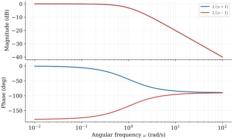
The familiar steady-state interpretation of $G(j\omega)$ assumes a stable system, but the algebraic evaluation can also be carried out for an unstable transfer function. This matters in feedback design because an unstable open loop may become stable after the loop is closed. Compare a stable real pole at $-a$ with an unstable one at $+a$, where $a\gt 0$.

$$ G_{\mathrm{s}}(s)=\frac{1}{s+a},\qquad G_{\mathrm{u}}(s)=\frac{1}{s-a},\qquad a\gt 0. $$

Time-domain stability concerns whether natural modes decay. The factor $1/(s-a)$ has the growing mode $e^{at}$, so a standalone sinusoidal experiment need not settle. Nevertheless, $G(j\omega)$ is an algebraic complex number wherever the denominator is nonzero. In feedback design the plant or controller may be unstable while the complete interconnection is stable. This motivates asking whether open-loop frequency information can determine closed-loop stability. A right-half-plane zero, such as $s-a$, is distinct from an unstable pole.

The unstable-pole vector

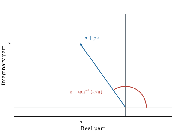
To evaluate the unstable example, first locate the denominator $j\omega-a$ in the complex plane. At positive frequency it lies in the second quadrant. Its reciprocal has the opposite angle, so the quadrant choice determines the correct continuous phase branch.

$$ \begin{aligned}j\omega-a&=-a+j\omega,\\|j\omega-a|&=\sqrt{a^2+\omega^2},\\\arg(j\omega-a)&=\pi-\tan^{-1}(\omega/a).\end{aligned} $$

For positive frequency, the denominator vector lies in quadrant II. It begins along the negative real axis and moves toward the positive imaginary direction. The numerator has phase zero; taking the reciprocal therefore negates this continuous denominator angle. Choosing the correct quadrant is essential: a one-argument arctangent alone would put this vector in the wrong quadrant.

Equal magnitudes, different phases

The denominator vectors for the stable and unstable poles have equal lengths at every frequency. Their angles, however, differ because their horizontal components have opposite signs. Thus magnitude alone cannot distinguish these two pole locations.

$$ |G_{\mathrm{s}}(j\omega)|=|G_{\mathrm{u}}(j\omega)|=\frac{1}{\sqrt{a^2+\omega^2}},\qquad \angle G_{\mathrm{u}}(j\omega)=-\pi+\tan^{-1}\!\frac{\omega}{a}. $$

For $\omega\ll a$, the magnitude approaches $1/a$. For $\omega\gg a$, it approaches $1/\omega$, giving a $-20$ dB/decade slope. The stable-pole phase moves from $0$ to $-90^\circ$; the unstable-pole phase, on the continuous branch used here, moves from $-180^\circ$ to $-90^\circ$. At $\omega=a$, their phases are $-45^\circ$ and $-135^\circ$. The straight-line phase approximation spans $0.1a$ to $10a$. The curves are normalized to $a=1$.

The closed-loop characteristic equation

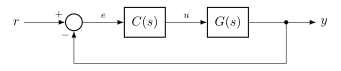
Since phase contains information that magnitude alone misses, we seek a stability test using the complete complex response. For negative unity feedback, the relevant roots are those of the closed-loop characteristic equation. Write the loop transfer function as $L(s)=C(s)G(s)=n(s)/d(s)$ to identify that equation.

$$ L(s)=C(s)G(s)=\frac{n(s)}{d(s)},\qquad T(s)=\frac{L(s)}{1+L(s)}=\frac{n(s)}{d(s)+n(s)}. $$

The roots of $d$ are open-loop poles. The roots of $d+n$ are closed-loop characteristic roots. The algebra preserves the numerator before cancellations, but an apparent cancellation must not hide an unstable internal mode. These notes assume a well-posed negative-feedback interconnection and no hidden unstable cancellations. Use a coprime representation when interpreting the root counts.

Derive the feedback transfer function

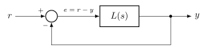
The characteristic denominator follows directly from the signal equations in the block diagram. If $r$ is the reference, $y$ is the output, and $e=r-y$ is the error, the forward path gives $y=Le$. Eliminating $e$ yields the closed-loop transfer function and shows why $d+n$ determines its characteristic roots.

$$ \begin{aligned}e&=r-y,\\y&=Le=L(r-y),\\(1+L)y&=Lr,\\T=\frac{y}{r}&=\frac{L}{1+L}.\end{aligned} $$

The error subtracts the measured output from the reference. Substitute the error into the forward path and collect the terms multiplying $y$. With $L=n/d$, multiplying numerator and denominator by $d$ yields $T=n/(d+n)$. Negative feedback changes the characteristic denominator from $d$ to $d+n$, while retaining the finite zeros before cancellations. The question is now how to count right-half-plane roots of $d+n$ without solving for all of them.

Complex mappings and winding

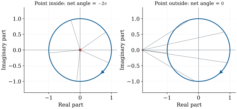
We could solve $d+n=0$ directly, but a geometric method can count unstable roots without locating each one. To develop it, let $s$ move around a closed contour and observe the image of a simple factor $s-z$. The total change in its continuous angle records whether the contour surrounds $z$.

$$ \Delta_\Gamma\arg(s-z)=0\quad\text{if }z\text{ lies outside a simple contour }\Gamma. $$

The vector $s-z$ may rotate forward and backward even when its net rotation is zero. Track the continuous angle around the complete path; comparing only the principal angles at the start and end loses whole turns. The picture shows a clockwise contour. A point on the contour is excluded from this argument because the vector would become zero.

A zero and a pole contribute opposite signs

When the zero lies inside a clockwise contour, the vector completes one clockwise turn. A pole contributes a reciprocal factor, which reverses that angular change. These opposite contributions are the basis of the argument principle.

$$ \Delta_\Gamma\arg(s-z)=-2\pi,\qquad \Delta_\Gamma\arg\!\left(\frac{1}{s-p}\right)=+2\pi. $$

These equations apply when the indicated zero or pole lies inside a simple clockwise contour. Multiplicity matters: a double zero contributes $-4\pi$ and a double pole contributes $+4\pi$. Factors outside the contour contribute zero.

Add the phase of every factor

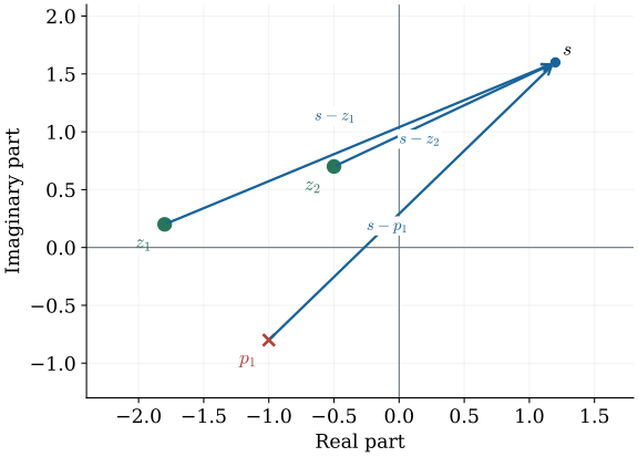
A general rational function is a product of the same elementary factors. Its angle is therefore the sum of the zero-factor angles minus the sum of the pole-factor angles. Over a complete traversal, only the enclosed roots contribute a net turn.

$$ \begin{aligned}F(s)&=k\frac{\prod_i(s-z_i)}{\prod_k(s-p_k)},\\\arg F(s)&=\arg k+\sum_i\arg(s-z_i)\\&\hspace{9mm}-\sum_k\arg(s-p_k).\end{aligned} $$

Each numerator factor is a vector from a zero to the moving point $s$; each denominator factor is a vector from a pole. Multiply magnitudes and add numerator angles, then subtract denominator angles. Over the complete clockwise contour, outside factors contribute zero net angle. Each enclosed zero contributes $-2\pi$ and each enclosed pole contributes $+2\pi$. A constant gain changes the starting angle but has zero net change.

Apply the argument principle to one plus the loop

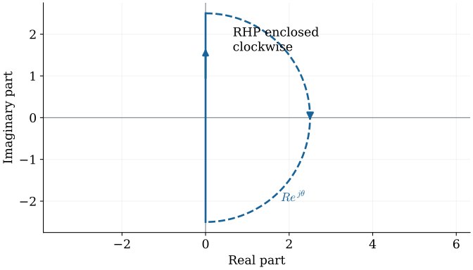
To turn this root count into a feedback stability test, apply it to $F(s)=1+L(s)$. Its numerator is the closed-loop characteristic polynomial, while its denominator contains the open-loop poles. The resulting net phase change relates a known open-loop pole count to the unknown closed-loop root count.

$$ F(s)=1+L(s)=\frac{d(s)+n(s)}{d(s)},\qquad \Delta_\Gamma\arg F=2\pi(P-Z). $$

Here $P$ counts poles of $F$ inside the contour and $Z$ counts its zeros, including multiplicities. A nonzero constant gain has no net phase change around a closed path, even if its fixed phase is not zero. The formula assumes no pole or zero lies on the contour. For a contour enclosing the right half-plane, $P$ becomes the number of unstable open-loop poles and $Z$ the number of unstable closed-loop characteristic roots.

Which zeros and poles are being counted?

The meaning of the zeros in this calculation deserves care. They are zeros of $1+L$, rather than transmission zeros of $L$. With a contour enclosing the right half-plane, these zeros are precisely the unstable closed-loop characteristic roots that the stability test must count.

$$ \begin{aligned}F(s)&=\frac{d(s)+n(s)}{d(s)},\\F(s)=0&\ \Longleftrightarrow\ d(s)+n(s)=0,\\\Delta\arg F&=-2\pi Z+2\pi P.\end{aligned} $$

The zeros in the argument-principle calculation are zeros of $F=1+L$, not zeros of $L$. They are the closed-loop characteristic roots. The poles of $F$ are the open-loop poles, using a coprime loop representation. Enclosing the right half-plane makes $P$ the unstable open-loop pole count and $Z$ the unstable closed-loop pole count. Assume no roots on the contour and no hidden unstable cancellation.

The stability target

The stability objective can now be stated as a target phase change. We require no right-half-plane closed-loop roots, so set $Z=0$ in the argument-principle relation. The required net rotation then depends on how many unstable poles the open loop already contains.

$$ Z=0\quad\Longleftrightarrow\quad \Delta_\Gamma\arg(1+L)=2\pi P. $$

For a stable open loop, $P=0$, the required net phase change is zero. With one unstable open-loop pole, $P=1$, the required net phase change is $2\pi$. This is a root-count statement, not a measure of how far the design is from instability. Boundary roots must be checked separately; they are not asymptotically stable.

Perspective

The argument principle converts the closed-loop stability question into a net rotation of $1+L$. For a clockwise right-half-plane contour, that rotation is $2\pi(P-Z)$. Once $P$ is known, measuring the rotation determines $Z$. The next geometric step is to read the same rotation from encirclements of $-1$ by the loop response itself.

The next lecture constructs the complete Nyquist contour and applies the resulting encirclement criterion to worked examples.

References

Norman S. Nise, Control Systems Engineering, 6th ed., Wiley, 2011.

• §5.2: Feedback block diagrams.
• §10.1: Frequency response.
• §10.3: Nyquist criterion and the argument principle.