Lecture 5: The Inverse Laplace Transform

Lecture 4 took us from an ODE to an algebraic equation and showed how to solve it for $Y(s)$. This lecture completes the round trip: it recovers the time-domain signal $y(t)$ from its transform. The key technique is partial fraction expansion, which breaks a complicated transform into simple pieces that we can look up in the table of transform pairs. We then use the method to solve first-order ODEs, connect ODEs to transfer functions, and define the DC gain, with Python and MATLAB code along the way.

Modularity and decomposition

The table of common transform pairs from Lecture 4 contains only simple, low-order terms such as $1/(s+a)$ and $\omega/((s+a)^2+\omega^2)$. A realistic transform, a ratio of two polynomials $G(s) = B(s)/A(s)$, rarely appears in the table as is. The strategy is to break it into small blocks,

each of which is an elementary pair. Because the Laplace transform is linear, the inverse transform of the sum is the sum of the inverse transforms. How we expand depends on the roots of $A(s)$. We show the strategy for each common case with an example. (We assume $G$ is strictly proper, with numerator degree lower than denominator degree. If not, first divide the polynomials.)

Real and distinct roots

Consider

The coefficients $K_i$ are called residues. To find $K_1$, multiply both sides by $s$ and let $s\to0$. Every term on the right vanishes except $K_1$:

In the same way,

This is often called the cover-up method: cover the factor of interest in the denominator and evaluate the rest at its root. With the table,

Symbolic tools do the same expansion:

# Python
import sympy
s = sympy.symbols('s')
G = 32/s/(s+4)/(s+8)
print(sympy.apart(G))        # 1/(s + 8) - 2/(s + 4) + 1/s

% MATLAB
syms s
G = 32/s/(s+4)/(s+8);
partfrac(G)

Real and repeated roots

A repeated root needs one term for each power:

$K_1$ and $K_3$ come from cover-up:

For $K_2$, multiplying by $(s+2)^2$ gives $(s+2)^2G(s) = K_1(s+2)^2/(s+1) + K_2(s+2) + K_3$. Differentiating once with respect to $s$ removes $K_3$ and isolates $K_2$ at $s=-2$:

Using $\mathcal{L}\{te^{-at}\} = 1/(s+a)^2$,

sympy.apart(2/(s+1)/(s+2)**2) returns -2/(s + 2) - 2/(s + 2)**2 + 2/(s + 1), confirming the result.

Complex roots

Complex roots come in conjugate pairs. Rather than splitting them into two complex terms, keep the quadratic factor and complete the square, so that the result matches the damped sine and cosine pairs. For example,

Cover-up gives $K_1 = 3/5$. Matching coefficients of $s^2$ and $s$ in $3 = K_1(s^2+2s+5) + (K_2s+K_3)s$ gives $K_2 = -3/5$ and $K_3 = -6/5$. Completing the square, $s^2+2s+5 = (s+1)^2+2^2$, so

This case is the one that produces oscillation. Lecture 7 uses exactly this pattern to derive the underdamped step response.

Solving first-order ODEs

Example 1: step input. Let $a\gt 0$, $b\gt 0$ and $y(0) = y_0\in\mathbb{R}$, and solve

With $\mathcal{L}\{\dot y\} = sY(s) - y(0)$, the ODE becomes $sY(s) - y_0 = -aY(s) + b/s$, so

The inverse transform is immediate:

The first term is the free response to the initial condition, which decays. The second is the forced response to the step, which rises to $b/a$.

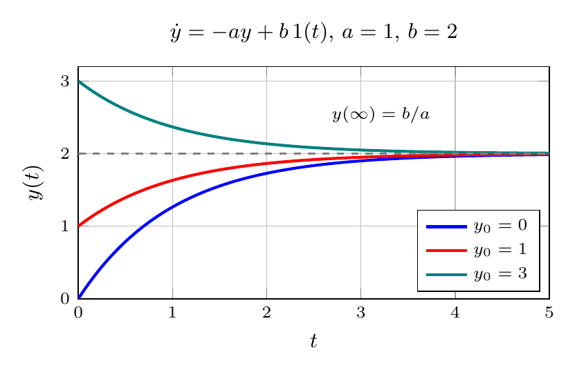
Two observations. From the ODE itself, at steady state $\dot y = 0$ and so $y(\infty) = b/a$. The final value theorem gives the same answer without solving anything:

Example 2: impulse input. Now solve $\dot y(t) = -ay(t) + b\,\delta(t)$ with $y(0) = y_0$. Since $\mathcal{L}\{\delta\} = 1$,

The initial value theorem gives $y(0^+) = \lim_{s\to\infty}sY(s) = y_0 + b$. What does the impulse do? It instantly moves the state from $y_0$ to $y_0+b$, and the system then responds freely from the new initial condition. An impulse input is equivalent to a jump in the initial condition.

Connecting the two domains: transfer functions

Return to the general $n$th-order ODE of Lecture 3,

now with all initial conditions zero: $y(0) = \dot y(0) = \cdots = y^{(n-1)}(0) = 0$. Applying the differentiation property term by term,

so

This is the transfer function. Its vocabulary:

• $A(s) = 0$ is the characteristic equation (C.E.).
• The roots of the C.E. are the poles of $G(s)$.
• The roots of $B(s) = 0$ are the zeros of $G(s)$.
• $m\le n$ is the realizability condition: a physical system cannot respond to a pure derivative of its input without limit.
• $G(s)$ is proper if $n\ge m$ and strictly proper if $n\gt m$.

For example, a pure gain $G_1(s) = K$ is proper, and a first-order lag $G_2(s) = k/(s+a)$ is strictly proper.

In Python, the control package represents transfer functions directly:

import control as co
import matplotlib.pyplot as plt
import numpy as np

num = [1, 2]                     # numerator coefficients:   s + 2
den = [1, 2, 3]                  # denominator coefficients: s^2 + 2s + 3
sys_tf = co.tf(num, den)
print(sys_tf)
print('poles =', co.poles(sys_tf), ' zeros =', co.zeros(sys_tf))

T, yout = co.step_response(sys_tf)
plt.plot(T, yout); plt.grid(True); plt.xlabel('Time (sec)'); plt.ylabel('y'); plt.show()

# responses to other inputs
u1 = 2 * np.ones_like(T)         # a constant input of 2
u2 = np.sin(T)                   # a sinusoidal input
T, yout_u1 = co.forced_response(sys_tf, T, u1)
T, yout_u2 = co.forced_response(sys_tf, T, u2)

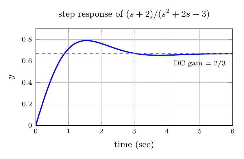
The poles are $-1\pm j\sqrt2$ and the zero is $-2$. The step response is shown below.

The DC gain

The DC gain is the ratio of a stable system’s output to its input after all transients have decayed, for a constant input. The final value theorem gives it directly. For a unit step input, $Y(s) = G(s)/s$, so

For $G_1(s) = K$ the DC gain is $K$, and for $G_2(s) = k/(s+a)$ it is $k/a$, which agrees with the ODE solution $b/a$ found above. For the Python example, $G(0) = 2/3$, the dashed line in the figure.

% MATLAB
s = tf('s');
G = (2*s+3)/(4*s^2+3*s+1);
dcgain(G)                        % 3

# Python
import control as co
s = co.tf('s')
G = (2*s+3)/(4*s**2+3*s+1)
print(co.dcgain(G))              # 3.0

A warning. The definition requires a stable system. Consider $Y_2(s) = 3/(s-2)$ from Lecture 4:

H = co.tf([0, 3], [1, -2])
print(co.dcgain(H))              # -1.5
T, yout = co.step_response(H)
print(yout)                      # grows without bound

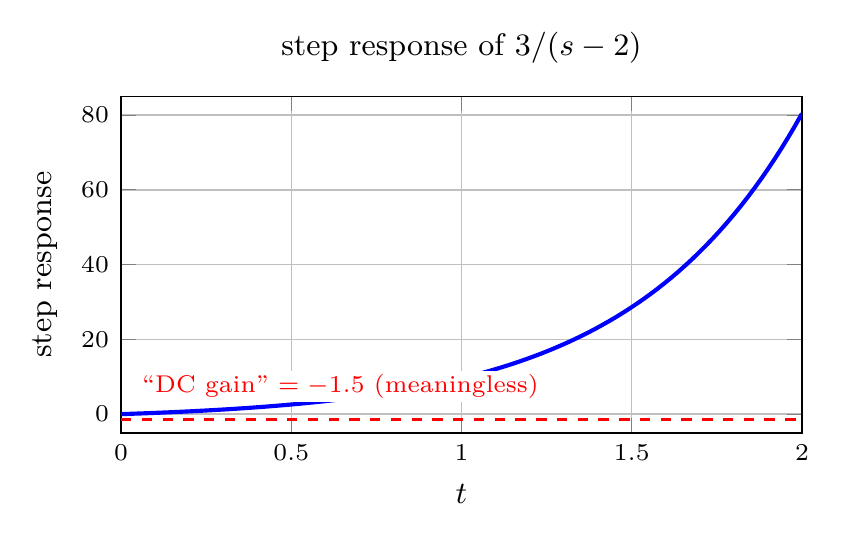
The software returns $G(0) = -1.5$ without complaint, but the step response grows exponentially and never settles. The number $-1.5$ is meaningless. As with the final value theorem, check stability before trusting a DC gain.

Summary and outlook

• Partial fraction expansion splits $B(s)/A(s)$ into table entries. Residues of distinct roots come from cover-up; repeated roots need derivatives; complex pairs are handled by completing the square.
• First-order ODEs: $y(t) = e^{-at}y_0 + \frac ba(1-e^{-at})$ for a step; an impulse acts like a jump in the initial condition.
• With zero initial conditions, an ODE becomes a transfer function $G(s) = B(s)/A(s)$, with poles, zeros, and the notions of proper and strictly proper.
• The DC gain is $G(0)$, valid only for stable systems.

This completes the review part of the course. We now have the tools to analyze how a system responds in time. The next lecture starts with the simplest cases: first- and second-order systems, and how the locations of their poles determine the response.

References

• N. S. Nise, Control Systems Engineering, 6th ed.: §2.2 Laplace Transform Review (p. 35), in particular the partial-fraction cases 1–3 (roots real and distinct, real and repeated, complex); §2.3 The Transfer Function (p. 44); §4.2 Poles, Zeros, and System Response (p. 162).
• X. Chen and M. Tomizuka, Introduction to Modern Controls, with Illustrations in MATLAB and Python: §3.2 Inverse Laplace Transform and Partial Fraction Expansion (p. 39); §3.3 From Laplace Transform to Transfer Functions (p. 41).