Lecture 10: Stability Analysis: the Routh-Hurwitz Approach

The last four lectures studied the transient response: how fast a system responds, how much it overshoots, and how extra poles and zeros change the picture. All of that assumed the response settles at all. This lecture makes that assumption precise. We define stability, relate it to pole locations, and learn the Routh-Hurwitz criterion, which counts the poles in the right half-plane from the coefficients of the characteristic polynomial alone, without computing any roots. This makes it the natural tool for finding the range of a controller gain that keeps a feedback loop stable.

Three goals of control design

A control system design pursues three goals:

1. a good transient response (Lectures 6–9),
2. stability (this lecture), and
3. small steady-state errors (Lecture 12).

Stability comes first in importance: an unstable system has no useful transient or steady state. Recall that the total response is

$$y_{\text{total}}(t) = y_{\text{forced}}(t) + y_{\text{natural}}(t).$$

Definitions

Based on the natural response.

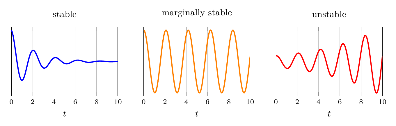
• A system is stable if the natural response approaches 0 as $t\to\infty$.
• A system is marginally stable if the natural response remains constant or oscillates and is bounded.
• A system is unstable if the natural response approaches $\infty$ as $t\to\infty$.

Based on the total response.

• A system is bounded-input, bounded-output (BIBO) stable if every bounded input yields a bounded output.
• A system is BIBO unstable if some bounded input produces an unbounded output.

The two views agree for stable and unstable systems but differ for marginally stable ones. An undamped oscillator has a bounded natural response, yet a bounded sinusoidal input at its natural frequency causes resonance: the output amplitude grows without bound. A marginally stable system is therefore BIBO unstable.

In terms of poles. For a closed-loop system $T(s) = G(s)/(1+G(s)H(s))$, the definitions translate into pole locations:

• Stable if all closed-loop poles are in the open left half-plane (LHP).
• Marginally stable if there are poles on the imaginary axis (a conjugate pair of imaginary poles, none repeated) and the rest are in the LHP.
• Unstable if there is at least one pole in the right half-plane (RHP), or a repeated pole on the imaginary axis.

Note that these are the poles of the closed loop, the roots of $1 + G(s)H(s) = 0$, not the poles of the open-loop transfer function $G(s)H(s)$. In the literature, a polynomial (or a matrix $A$) whose roots (eigenvalues) all have negative real parts is called Hurwitz, so “the system is Hurwitz” means it is stable.

Quick checks

A few observations about the closed-loop denominator settle many cases without any work.

1. If there is at least one sign change among the coefficients, the system is unstable. For example, $s^2 - 4s + 4 = (s-2)^2$ has two poles at $+2$.
2. If a power of $s$ is missing, the system is marginally stable or unstable. For example, $s^2 + 4$ has poles at $\pm2j$ (marginally stable) and $s^2 - 1$ has poles at $\pm1$ (unstable). A missing constant term just means a pole at the origin: $s^3 + s^2 + s = s(s^2+s+1)$.
3. If all coefficients have the same sign and no power is missing, the checks are inconclusive. For polynomials of degree three or more, the roots can still lie in the RHP. For example, $s^5 + 3s^4 + s^3 + 2s^2 + 3s + 1$ has positive coefficients, but two of its roots, $0.46\pm0.94j$, are in the RHP. (The annotated slide says one; the Routh table below shows two sign changes.)

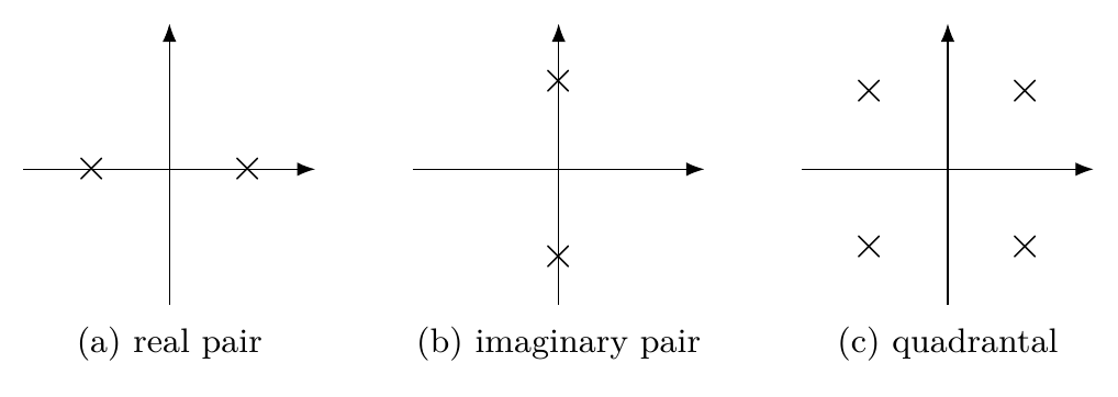
Rule 2 reflects a symmetry. A missing power typically means the polynomial has a factor with roots placed symmetrically about the origin: (a) a real pair $\pm\sigma$, (b) an imaginary pair $\pm j\omega$, or (c) a quadrantal quadruple $\pm\sigma\pm j\omega$. Of these, (b) is the best case (marginal stability); (a) and (c) always put a root in the RHP.

Case 3 is where we need a real test.

The Routh-Hurwitz criterion

The Routh-Hurwitz criterion determines how many closed-loop poles lie in the LHP, in the RHP and on the imaginary axis, though not where exactly. It is useful for deciding stability by hand, and, more importantly, for finding the range of a parameter that keeps a system stable.

Step 1: build the Routh table. For a closed-loop transfer function

$$G_{CL}(s) = \frac{N(s)}{a_4s^4 + a_3s^3 + a_2s^2 + a_1s + a_0},$$

write the coefficients in the first two rows, alternating, and compute each following row from the two rows above it:

$$\begin{array}{c|ccc} s^4 & a_4 & a_2 & a_0\\ s^3 & a_3 & a_1 & 0\\ s^2 & b_1 = \dfrac{a_3a_2 - a_4a_1}{a_3} & b_2 = \dfrac{a_3a_0 - a_4\cdot0}{a_3} = a_0 & 0\\ s^1 & c_1 = \dfrac{b_1a_1 - a_3b_2}{b_1} & 0 & 0\\ s^0 & d_1 = b_2 & 0 & 0 \end{array}$$

Each entry is minus the determinant of a $2\times2$ matrix formed from the first column and the next column of the two rows above, divided by the first entry of the row directly above. Any row may be multiplied by a positive constant to simplify the arithmetic.

Step 2: interpret the table. The number of sign changes in the first column, $a_4\to a_3\to b_1\to c_1\to d_1$, equals the number of poles in the RHP. In particular,

$$\text{no sign changes} \iff \text{no poles in the RHP} \iff \text{stable}$$

(provided no special case, described below, occurs).

Example: a unity-feedback loop

Assuming unity negative feedback, determine the stability of the loop with

$$G(s) = \frac{1000}{(s+2)(s+3)(s+5)}, \qquad H(s) = 1 .$$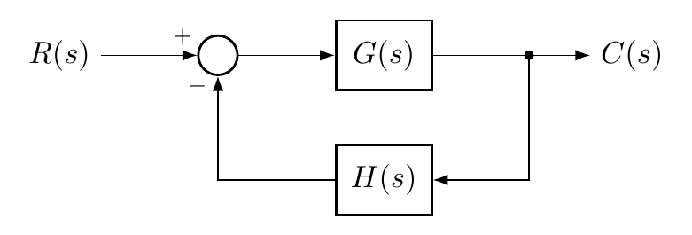

The open-loop poles $-2, -3, -5$ are all stable. The closed loop is another matter. Its characteristic equation $1 + G(s) = 0$ is

$$(s+2)(s+3)(s+5) + 1000 = s^3 + 10s^2 + 31s + 1030 = 0 .$$

All coefficients are positive, so the quick checks are inconclusive. The Routh table, with the $s^2$ row divided by 10, is

$$\begin{array}{c|cc} s^3 & 1 & 31\\ s^2 & 1 & 103\\ s^1 & -72 & 0\\ s^0 & 103 & 0 \end{array}$$

The first column $1, 1, -72, 103$ changes sign twice, so the closed loop has two poles in the RHP and is unstable. (Numerically, the closed-loop poles are $-13.41$ and $1.71\pm8.60j$.) The gain of 1000 is too high; the last example of this lecture shows how to find the largest acceptable gain.

Special case 1: a zero in the first column

If the first entry of a row is zero while the rest of the row is not, the next row would require dividing by zero. Replace the zero with a small number $\epsilon$, finish the table, and examine the signs as $\epsilon\to0$ from either side (the result is the same).

Example.

$$G_{CL}(s) = \frac{10}{s^5 + 2s^4 + 3s^3 + 6s^2 + 5s + 3}.$$$$\begin{array}{c|ccc} s^5 & 1 & 3 & 5\\ s^4 & 2 & 6 & 3\\ s^3 & \bcancel{0}\ \epsilon & \tfrac72 & 0\\ s^2 & \dfrac{6\epsilon-7}{\epsilon} & 3 & 0\\ s^1 & \dfrac{42\epsilon - 49 - 6\epsilon^2}{12\epsilon - 14} & 0 & 0\\ s^0 & 3 & 0 & 0 \end{array}$$

As $\epsilon\to0^+$, the first column has signs $+,+,+,-,+,+$ (the $s^1$ entry tends to $49/14 \gt 0$). There are two sign changes, so two RHP poles: the system is unstable. With $\epsilon\to0^-$ the signs are $+,+,-,+,+,+$, again two changes. (Roots: $0.34\pm1.51j$, $-1.67$, $-0.51\pm0.70j$.)

Special case 2: an entire row of zeros

An entire row of zeros means the polynomial has a factor with roots symmetric about the origin, the pole pairs of the quick-check figure. Proceed as follows.

1. Form the auxiliary polynomial $P(s)$ from the row above the row of zeros. It is an even polynomial whose powers drop by two from row to row.
2. Differentiate it with respect to $s$.
3. Replace the row of zeros with the coefficients of $dP/ds$.
4. Complete the Routh table and interpret it.

The roots of $P(s)$ are exactly the symmetric roots. Sign changes from the auxiliary row downward count the symmetric roots in the RHP; by symmetry, the same number lies in the LHP, and the remaining symmetric roots are on the imaginary axis.

Example.

$$G(s) = \frac{1}{s^5 + 7s^4 + 6s^3 + 42s^2 + 8s + 56}.$$

The $s^4$ row $7, 42, 56$ divided by 7 is $1, 6, 8$, identical to the $s^5$ row, so the $s^3$ row is all zeros. The auxiliary polynomial is

$$P(s) = s^4 + 6s^2 + 8, \qquad \frac{dP}{ds} = 4s^3 + 12s,$$

and the table becomes

$$\begin{array}{c|ccc} s^5 & 1 & 6 & 8\\ s^4 & 1 & 6 & 8\\ s^3 & \bcancel{0}\ 1 & \bcancel{0}\ 3 & 0\\ s^2 & 3 & 8 & 0\\ s^1 & \tfrac13 & 0 & 0\\ s^0 & 8 & 0 & 0 \end{array}$$

(the $s^3$ row is $4, 12$ divided by 4). There are no sign changes, so no RHP poles. The four roots of $P(s)$ are symmetric about the origin; none is in the RHP, so none is in the LHP either, and all four lie on the imaginary axis. Indeed, $P(s) = (s^2+2)(s^2+4)$ gives $s = \pm j\sqrt2$ and $\pm2j$. The fifth pole, from the upper part of the table, is in the LHP (it is $-7$). The imaginary poles are distinct, so the system is marginally stable.

Finding a stabilizing range of gain

The most useful application of the Routh table is to design problems. Consider unity feedback around

$$G(s) = \frac{K}{s(s+7)(s+11)} = \frac{K}{s^3 + 18s^2 + 77s}.$$

For which $K$ is the closed loop stable, unstable, or marginally stable? The closed-loop characteristic polynomial is $s^3 + 18s^2 + 77s + K$, and

$$\begin{array}{c|cc} s^3 & 1 & 77\\ s^2 & 18 & K\\ s^1 & \dfrac{1386 - K}{18} & 0\\ s^0 & K & 0 \end{array}$$

• Stable if every first-column entry is positive: $1386 - K \gt 0$ and $K \gt 0$, that is, $0 \lt K \lt 1386$.
• Unstable if $K \gt 1386$ (two sign changes, two RHP poles) or $K \lt 0$ (one sign change, one RHP pole).
• Marginally stable at $K = 1386$. The $s^1$ row vanishes, the auxiliary polynomial is $18s^2 + 1386$, and the closed loop has poles at $s = \pm j\sqrt{77} = \pm 8.77j$. The loop oscillates at $\omega = \sqrt{77}\approx8.77$ rad/s.

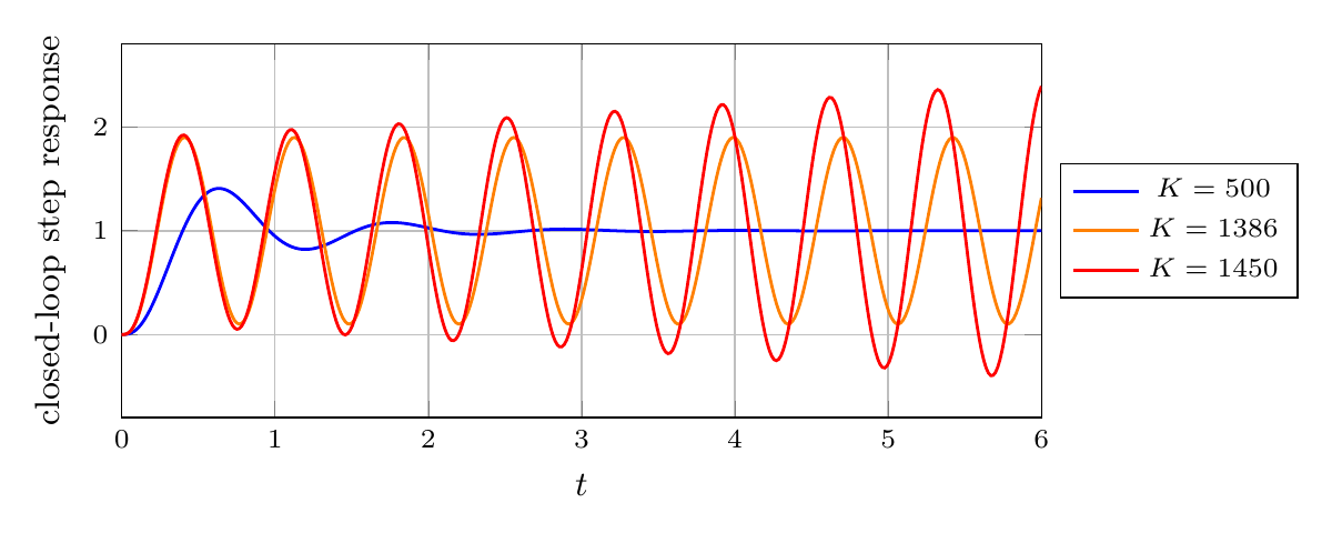
The crossing point $K = 1386$, $\omega = 8.77$ rad/s is exactly where the root locus of Lecture 13 will cross the imaginary axis; the Routh table is how we will compute such crossings.

A note on state-space models

If the closed loop is given in state space with matrix $A$, its poles are the eigenvalues of $A$, the roots of $\det(sI - A) = 0$. The Routh-Hurwitz criterion applies to this characteristic polynomial in exactly the same way. A single eigenvalue with a positive real part makes the system unstable. (State space is the subject of ME 547.)

Summary and outlook

• Stability depends on the closed-loop poles: all in the LHP means stable (BIBO stable); any in the RHP means unstable; distinct imaginary poles mean marginally stable (BIBO unstable).
• Quick checks: a sign change means unstable, a missing power means not asymptotically stable.
• The Routh table counts RHP poles by sign changes in its first column. A zero in the first column is handled with $\epsilon$; a row of zeros signals symmetric roots and is handled with the auxiliary polynomial.
• With a gain $K$ in the table, the first column gives the stabilizing range, and the auxiliary polynomial at the boundary gives the oscillation frequency.

Stability tells us whether a loop works; it does not tell us how well. The next lecture puts stability to work on a concrete problem: using PD control to stabilize an unstable plant.

References

• N. S. Nise, Control Systems Engineering, 6th ed.: §6.1 Introduction (p. 302); §6.2 Routh-Hurwitz Criterion (p. 305); §6.3 Routh-Hurwitz Criterion: Special Cases (p. 308); §6.4 Routh-Hurwitz Criterion: Additional Examples (p. 314); §6.5 Stability in State Space (p. 320).
• X. Chen and M. Tomizuka, Introduction to Modern Controls, with Illustrations in MATLAB and Python: §8.2 Stability of LTI Systems (p. 144); §8.2.1 Method of Eigenvalue Locations (p. 144); §8.2.2 Routh-Hurwitz Criterion for Continuous-Time LTI Systems (p. 146).

Adapted from the ME 545 slides “Stability” (T. Chu, UW ME 545, 2024) and their annotations.