Lecture 13: The Root Locus Technique
Lecture 10 used the Routh table to find the range of gain that keeps a loop stable, and Lecture 12 showed how the gain sets the steady-state error. Both answers are about one value of $K$ at a time, or a boundary. A designer wants more: to see where all the closed-loop poles go as the gain changes, and so how stability, damping and speed change together. The root locus gives exactly that picture. This lecture defines it, derives the rules for sketching it by hand, and refines the sketch with break-away points, imaginary-axis crossings and departure angles. The lectures that follow use it as the main design tool of the time-domain part of the course.
Open loop, closed loop, and the gain $K$
Consider the feedback loop below, with an adjustable gain $K$ in the forward path.

- The open-loop transfer function (OLTF) is $KG(s)H(s)$.
- The closed-loop transfer function (CLTF) is $T(s) = \dfrac{KG(s)}{1 + KG(s)H(s)}$.
Writing $G = N_G/D_G$ and $H = N_H/D_H$,
$$\text{OLTF} = K\frac{N_G(s)N_H(s)}{D_G(s)D_H(s)}, \qquad T(s) = \frac{KN_G(s)D_H(s)}{D_G(s)D_H(s) + KN_G(s)N_H(s)} .$$Changing $K$ does not move the open-loop poles, but it does move the closed-loop poles, the roots of
$D_GD_H + KN_GN_H$. The root locus (RL) is the path of the closed-loop poles as $K$ varies, usually
from $0$ to $\infty$. In MATLAB it is drawn by rlocus, and in Python by
control.root_locus. It gives a qualitative picture of the loop’s performance and is the basis of
compensator design with PID and lead-lag controllers (Lectures 16–20).
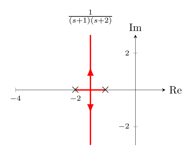
Example: a security camera. A pan-tilt camera tracking a moving subject has closed-loop transfer function
$$T(s) = \frac{k_1k_2}{s^2 + 10s + k_1k_2} = \frac{K}{s^2 + 10s + K}.$$The closed-loop poles are $s = -5\pm\sqrt{25 - K}$. For $0 \lt K \lt 25$ they are real and move toward each other from $0$ and $-10$; at $K = 25$ they meet at $-5$; for $K \gt 25$ they become complex, $-5\pm j\sqrt{K-25}$, and move vertically. The real part stays at $-5$, so the settling time does not change, while the overshoot grows with $K$. A single picture shows all of this at once:
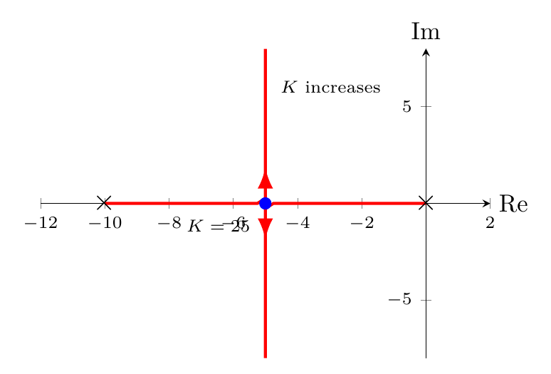
For a second-order loop we could solve the quadratic. For higher orders we need rules.
Review: magnitude and phase of a transfer function
The rules rest on evaluating a transfer function at a point of the complex plane. A factor $F(s) = s + a$ evaluated at $s = \sigma + j\omega$ is the complex number $(\sigma + a) + j\omega$: the vector from the point $-a$ to the point $s$. Its length is $|s + a|$ and its angle, measured counterclockwise from the positive real axis, is $\angle(s + a)$. A factor $1/(s + a)$ has the reciprocal length and the negative angle.
For a general transfer function
$$G(s) = \frac{(s+z_1)\cdots(s+z_m)}{(s+p_1)\cdots(s+p_n)} = \frac{\prod_{i=1}^m(s+z_i)}{\prod_{k=1}^n(s+p_k)},$$$$M = |G(s)| = \frac{\prod\text{zero lengths}}{\prod\text{pole lengths}} = \frac{\prod_{i=1}^m|s+z_i|}{\prod_{k=1}^n|s+p_k|},$$$$\theta = \angle G(s) = \sum\text{zero angles} - \sum\text{pole angles} = \sum_{i=1}^m\angle(s+z_i) - \sum_{k=1}^n\angle(s+p_k).$$The same computation underlies compensator design (Lectures 17–18) and, later, frequency-response analysis with Bode plots.
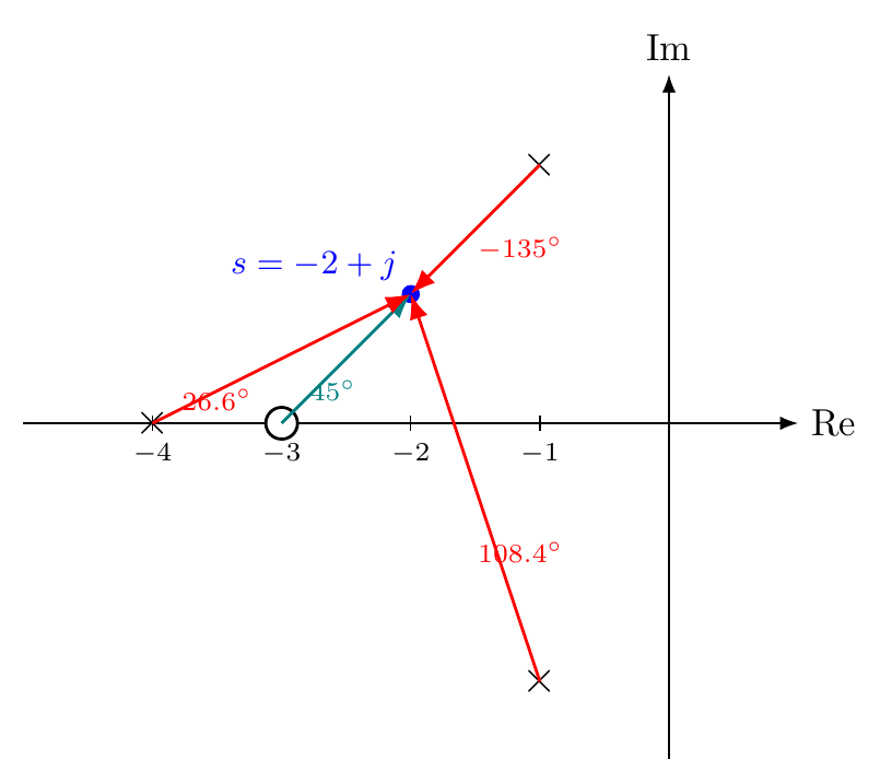
Example. Find the magnitude and phase of $G(s) = \dfrac{s+3}{(s+4)(s^2+2s+5)}$ at $s = -2+j$. The poles are $-4$ and $-1\pm2j$ and the zero is $-3$. Drawing the vectors to $s = -2+j$:
| from | vector | length | angle |
|---|---|---|---|
| zero $-3$ | $1 + j$ | $\sqrt2$ | $45^\circ$ |
| pole $-4$ | $2 + j$ | $\sqrt5$ | $26.6^\circ$ |
| pole $-1+2j$ | $-1 - j$ | $\sqrt2$ | $-135^\circ$ |
| pole $-1-2j$ | $-1 + 3j$ | $\sqrt{10}$ | $108.4^\circ$ |
Defining the root locus
A point $s_1$ is on the root locus if a closed-loop pole can sit there for some $K \gt 0$, that is, if
$$1 + KG(s_1)H(s_1) = 0 \quad\Longleftrightarrow\quad KG(s_1)H(s_1) = -1 .$$The number $-1$ has magnitude 1 and angle $180^\circ$ (plus any multiple of $360^\circ$). So $s$ is on the root locus if and only if it satisfies
$$\textbf{magnitude condition: } |KG(s)H(s)| = 1, \qquad \textbf{angle condition: } \angle G(s)H(s) = (2i+1)\,180^\circ,\ i\in\mathbb{Z}.$$The angle condition does not involve $K$ at all: it alone decides which points are on the locus. Once a point is known to be on the locus, the magnitude condition gives the gain that puts a pole there:
$$K = \frac{1}{|G(s)H(s)|} = \frac{\prod\text{pole lengths}}{\prod\text{zero lengths}} .$$In the example above, $\angle G(-2+j) = 45^\circ$, not an odd multiple of $180^\circ$, so $-2+j$ is not on the root locus of that system.
Sketching rules
Write the closed-loop characteristic equation as
$$1 + KG(s) = 0, \qquad G(s) = \frac{B(s)}{A(s)} = \frac{\prod_{i=1}^m(s - z_i)}{\prod_{i=1}^n(s - p_i)}, \qquad n\ge m\ge0,$$where $G$ now stands for the whole loop $GH$. The closed-loop poles solve $A(s) + KB(s) = 0$. We assume $K \gt 0$; a negative gain can be absorbed into $\tilde G(s) = -G(s)$.
1. Number of branches. $A(s) + KB(s)$ has degree $n$, so there are $n$ closed-loop poles, and as $K$ changes they trace out $n$ branches, one per closed-loop pole.
2. Symmetry. A physical system has real coefficients, so its closed-loop poles are real or come in complex-conjugate pairs. The root locus is symmetric about the real axis.
3. Starting and ending points. At the two extremes,
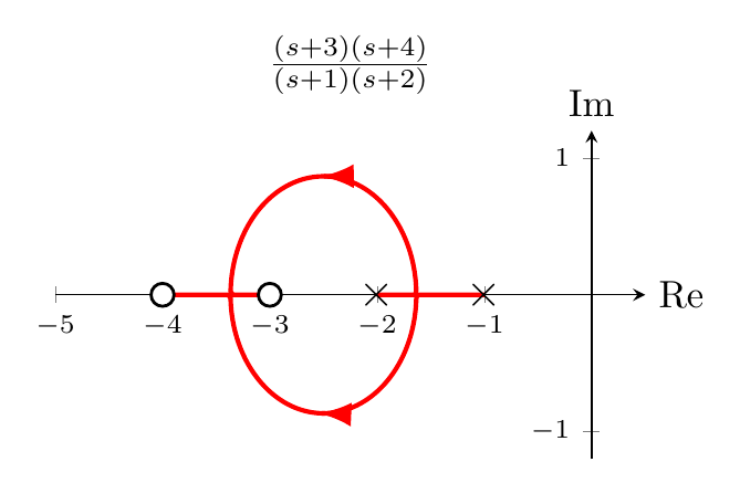
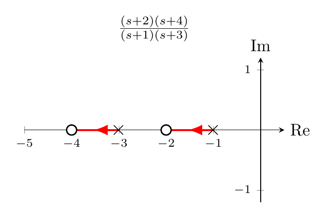
$$K = 0:\ A(s) = 0, \qquad K\to\infty:\ \tfrac1KA(s) + B(s) \to B(s) = 0 .$$The root locus begins at the open-loop poles and ends at the open-loop zeros. These three rules already fix the locus when $n = m$. For $G(s) = \frac{(s+3)(s+4)}{(s+1)(s+2)}$, the branches must leave $-1$ and $-2$ and arrive at $-3$ and $-4$, and symmetry allows only one way: the poles meet between $-1$ and $-2$, break away into a circle, and re-enter the real axis between $-3$ and $-4$. For $G(s) = \frac{(s+2)(s+4)}{(s+1)(s+3)}$, each pole simply slides left along the real axis to the neighbouring zero.
Poles and zeros at infinity. When $m \lt n$, there are more branches than finite zeros. Where do the extra branches end? A function has a zero at infinity if $G(s)\to0$ as $s\to\infty$. For example, $1/s^2$ has two zeros at infinity; formally
$$G(s) = \frac{1}{s^2} = \lim_{\rho\to\infty}\frac{\left(1 + \frac{s}{\rho}\right)^2}{s^2},$$with two zeros at $-\rho\to\infty$. Likewise, $G(s) = s = \lim_{\rho\to\infty} s/(1 + s/\rho)$ has a pole at infinity. Counting finite and infinite ones, every transfer function has as many poles as zeros. For instance, $K(s+1)/((s+2)(s+3)(s+5))$ has three finite poles, one finite zero, and two zeros at infinity. The $n - m$ extra branches go off to the zeros at infinity.
4. Real-axis segments. For $K \gt 0$, the root locus exists on the real axis to the left of an odd number of real open-loop poles and zeros. At a real test point, a complex-conjugate pair contributes angles that cancel, and a real pole or zero to the left contributes $0^\circ$. Each real pole or zero to the right contributes $180^\circ$, so the total is an odd multiple of $180^\circ$ exactly when their number is odd.
5. Asymptotes. Far from the origin, a point on the locus sees all poles and zeros at almost the same angle, and the characteristic equation behaves like $1 + K/(s - \alpha)^{n-m} = 0$ for some center $\alpha$. The angle condition then gives $(n - m)\,\angle(s - \alpha) = (2k+1)180^\circ$, so the $n - m$ branches approach straight-line asymptotes with
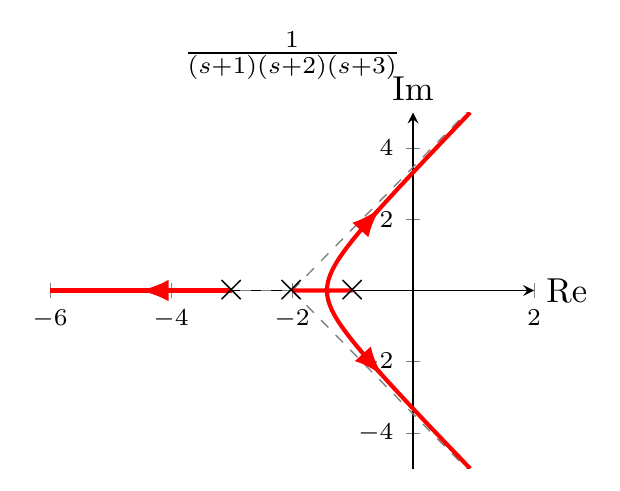
$$\text{angles } \theta_a = \frac{(2k+1)\,180^\circ}{n - m}, \quad k = 0, 1, \ldots, n-m-1, \qquad \text{centroid } \sigma_a = \frac{\sum\text{finite poles} - \sum\text{finite zeros}}{n - m}.$$For example, $1/((s+1)(s+2))$ has asymptotes at $\pm90^\circ$ from $-1.5$, and $1/((s+1)(s+2)(s+3))$ has asymptotes at $60^\circ$, $180^\circ$ and $300^\circ$ from $-2$:
Why the centroid formula holds. Write $A(s) = s^n + a_1s^{n-1} + \cdots$, so that the sum of the open-loop poles is $-a_1$. When $m \lt n - 1$, adding $KB(s)$ does not touch the $s^{n-1}$ coefficient, so the closed-loop poles $\rho_i$ have the same sum: $\sum\rho_i = \sum p_i$ for every $K$. As $K\to\infty$, $m$ of the closed-loop poles approach the zeros (sum $\sum z_i$) and the other $n - m$ recede along the asymptotes with center $\alpha$ (sum $(n-m)\alpha$). Hence $\sum p_i = (n - m)\alpha + \sum z_i$, which is the formula for $\sigma_a$. (When $m = n - 1$ there is a single asymptote along the negative real axis, and the centroid is not needed.)
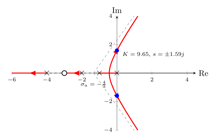
Example. Sketch the root locus of the unity-feedback system with
$$G(s) = \frac{s+3}{s(s+1)(s+2)(s+4)} .$$- Four branches, starting at $0, -1, -2, -4$; one ends at the zero $-3$, three go to infinity.
- Real-axis segments (left of an odd count): $[-1, 0]$ and $[-3, -2]$, and $(-\infty, -4]$.
- Asymptotes: $n - m = 3$, angles $60^\circ, 180^\circ, 300^\circ$, centroid $\sigma_a = \dfrac{(0 - 1 - 2 - 4) - (-3)}{3} = -\dfrac43$.
The branches from $0$ and $-1$ meet, break away, and bend toward the $\pm60^\circ$ asymptotes, crossing into the right half-plane. The branch from $-2$ moves to the zero at $-3$, and the branch from $-4$ runs to $-\infty$.
Refining the sketch
Three more calculations turn the sketch into an accurate plot:
- real-axis break-away and break-in points,
- the imaginary-axis crossing, and
- angles of departure and arrival at complex poles and zeros.
Break-away and break-in points
The break-away point is where two branches leave the real axis (the poles go from real to complex conjugate); the break-in point is where they return. Two methods find them.
(a) Maximize the gain. On the real axis, $K = -1/(G(\sigma)H(\sigma))$. Along a segment between two poles, $K$ rises from 0, reaches a maximum where the poles meet, and the poles then leave the axis. Break-away and break-in points therefore satisfy
$$\frac{dK}{d\sigma} = -\frac{d}{d\sigma}\frac{1}{G(\sigma)H(\sigma)} = 0 .$$(b) Transition method. Equivalently, without differentiating,
$$\sum_{i=1}^m\frac{1}{\sigma + z_i} = \sum_{k=1}^n\frac{1}{\sigma + p_k},$$where $-z_i$ and $-p_k$ are the zeros and poles.
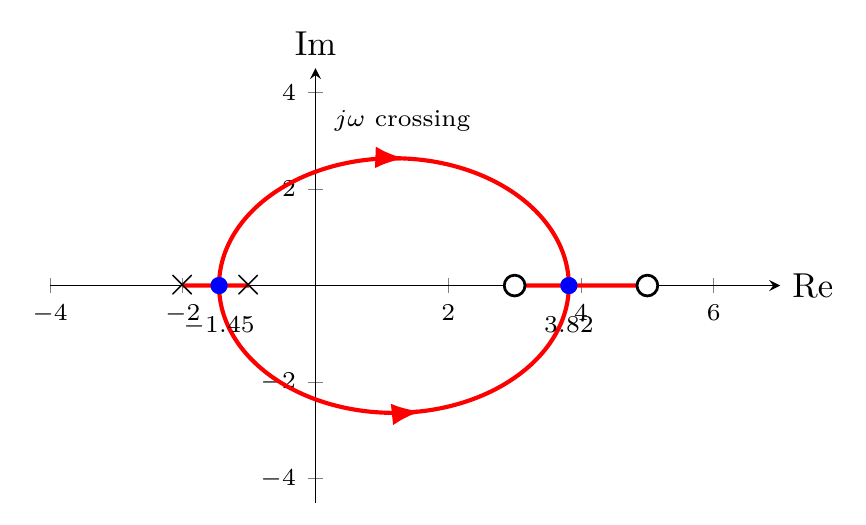
Example. $G(s) = \dfrac{(s-3)(s-5)}{(s+1)(s+2)}$. On the real axis,
$$K = -\frac{(\sigma+1)(\sigma+2)}{(\sigma-3)(\sigma-5)}, \qquad \frac{dK}{d\sigma} = 0 \ \Longrightarrow\ 11\sigma^2 - 26\sigma - 61 = 0 \ \Longrightarrow\ \sigma = -1.45,\ 3.82 .$$The transition method gives the same equation from $\frac{1}{\sigma-3} + \frac{1}{\sigma-5} = \frac{1}{\sigma+1} + \frac{1}{\sigma+2}$. The poles break away at $-1.45$ (with $K = 0.0086$), loop through the right half-plane, and break in at $3.82$ ($K = 29.0$) before moving to the zeros at $3$ and $5$.
Imaginary-axis crossings
The $j\omega$ crossing is the gain at which the closed loop changes from stable to unstable (or the reverse). Two methods work: the Routh table of Lecture 10 (a row of zeros at the critical gain), or substituting $s = j\omega$ into the characteristic equation and setting the real and imaginary parts to zero.
Example. For the sketch example above, $G(s) = \frac{s+3}{s(s+1)(s+2)(s+4)}$ and
$$T(s) = \frac{K(s+3)}{s^4 + 7s^3 + 14s^2 + (8 + K)s + 3K}.$$With $s = j\omega$:
$$\text{Re: } \omega^4 - 14\omega^2 + 3K = 0, \qquad \text{Im: } -7\omega^3 + (8 + K)\omega = 0 .$$The second gives $K = 7\omega^2 - 8$; substituting in the first gives $\omega^4 + 7\omega^2 - 24 = 0$, so $\omega^2 = 2.52$, $\omega = \pm1.59$ rad/s, and $K = 9.65$. The closed loop is stable for $0 \lt K \lt 9.65$. The Routh table gives the same result: its $s^1$ row vanishes at $K = 9.65$. These are the blue points in the sketch. For the break-away example, $(1+K)s^2 + (3 - 8K)s + (2 + 15K) = 0$ crosses the axis when $K = 3/8$, at $\omega = \pm2.35$.
Angles of departure and arrival
Near a complex open-loop pole, in which direction does the locus leave? Apply the angle condition to a test point $s$ very close to the pole $p_i$. Seen from $s$, every other pole and zero is at the same angle as seen from $p_i$, so $\angle(s - z_k)\approx\angle(p_i - z_k)$ and $\angle(s - p_j)\approx\angle(p_i - p_j)$ for $j\ne i$. The only unknown is the angle of the short vector from $p_i$ to $s$, the departure angle $\theta_{dep}$. The angle condition,
$$\sum_k\angle(p_i - z_k) - \sum_{j\ne i}\angle(p_i - p_j) - \theta_{dep} = 180^\circ,$$gives
$$\theta_{dep} = \sum_k\angle(p_i - z_k) - \sum_{j\ne i}\angle(p_i - p_j) - 180^\circ \pmod{360^\circ}.$$The arrival angle at a complex zero $z_i$ follows in the same way:
$$\theta_{arr} = \sum_k\angle(z_i - p_k) - \sum_{j\ne i}\angle(z_i - z_j) + 180^\circ \pmod{360^\circ}.$$For a pole (zero) of multiplicity $q$, $q$ branches leave (arrive), with $q\,\theta$ equal to the right side plus $360^\circ(l - 1)$, $l = 1, \ldots, q$.
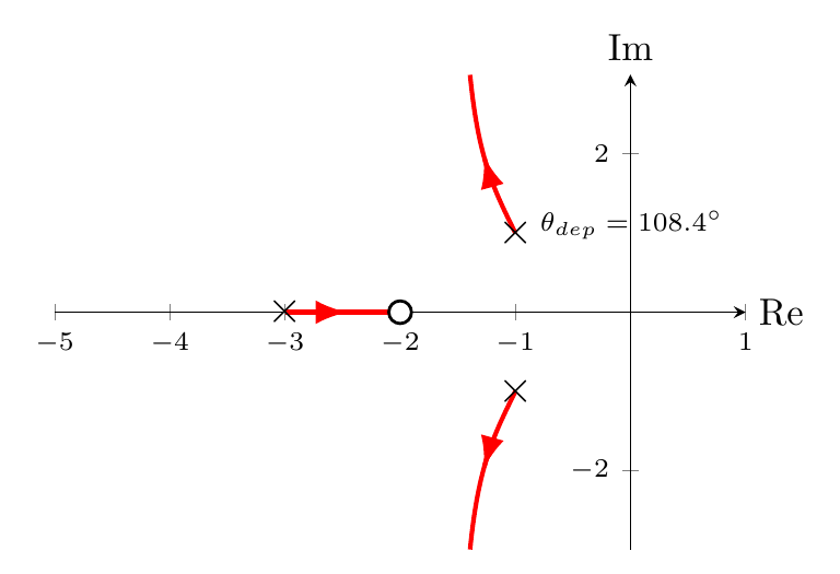
Example. $G(s) = \dfrac{s+2}{(s+3)(s^2+2s+2)}$, $H = 1$. At the pole $p = -1 + j$:
- angle from the zero $-2$: $\angle(1 + j) = 45^\circ$;
- angle from the pole $-3$: $\angle(2 + j) = 26.6^\circ$;
- angle from the conjugate pole $-1 - j$: $\angle(2j) = 90^\circ$.
The branch leaves the upper pole up and to the left, as the computed locus confirms. By symmetry, the lower branch departs at $-108.4^\circ$.
Lecture 14 works through several more departure and arrival problems, where these angles decide the shape of the whole locus.
The generalized root locus
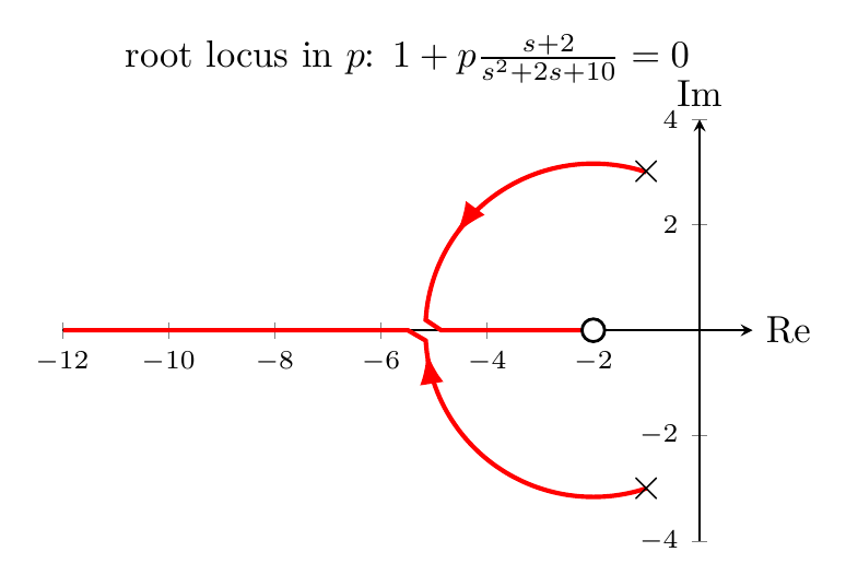
The root locus is usually drawn as a function of the gain $K$. What if $K$ is fixed and some other parameter varies? Consider
$$G(s) = \frac{10}{(s+2)(s+p)}, \qquad H(s) = 1,$$and let $p$ vary from $0$ to $\infty$. The closed-loop transfer function is
$$\frac{G}{1+G} = \frac{10}{s^2 + (p+2)s + 2p + 10} = \frac{10}{s^2 + 2s + 10 + p(s+2)} = \frac{\dfrac{10}{s^2+2s+10}}{1 + p\,\dfrac{s+2}{s^2+2s+10}} .$$The denominator has the standard form $1 + pG_{eq}(s)$ with $G_{eq}(s) = \dfrac{s+2}{s^2+2s+10}$, so all the sketching rules apply with $p$ in place of $K$. The branches start at $-1\pm3j$, circle around to meet on the real axis, and then one branch approaches the zero at $-2$ while the other goes to $-\infty$.
Summary and outlook
- The root locus is the path of the closed-loop poles as $K$ varies. It gives a qualitative picture of how stability and the transient response change with the gain.
- A point is on the locus if and only if $\angle G(s)H(s) = (2i+1)180^\circ$; the gain there is $K = \prod\text{pole lengths}/\prod\text{zero lengths}$.
- Sketching: $n$ branches, symmetric about the real axis, from the open-loop poles to the open-loop zeros (finite or infinite), on the real axis left of an odd count, with asymptotes at $(2k+1)180^\circ/(n-m)$ from $\sigma_a = (\sum p - \sum z)/(n - m)$.
- Refining: break-away/break-in from $dK/d\sigma = 0$, $j\omega$ crossings from the Routh table, and departure/arrival angles from the angle condition.
- The generalized root locus handles any parameter that enters the characteristic equation linearly.
The root locus can now be used to choose the gain, and the closed-loop pole locations, for a desired transient response. Before we do so, the next lecture takes a closer look at departure and arrival angles through a set of examples worked on the board.
References
- N. S. Nise, Control Systems Engineering, 6th ed.: §8.1 Introduction (p. 388); §8.2 Defining the Root Locus (p. 392); §8.3 Properties of the Root Locus (p. 394); §8.4 Sketching the Root Locus (p. 397); §8.5 Refining the Sketch (p. 402); §8.6 An Example (p. 411); §8.8 Generalized Root Locus (p. 419).
- X. Chen and M. Tomizuka, Introduction to Modern Controls, with Illustrations in MATLAB and Python: §8.2.2 Routh-Hurwitz Criterion (p. 146), for the imaginary-axis crossings. (The root locus itself is covered in Nise, Ch. 8, and in X. Chen, “Essentials of root locus,” course notes, 2025.)