Lecture 16: Pole Locations and the Second-Order Response
Root-locus design, the subject of the next lectures, means choosing the gain (and the compensator) so that closed-loop poles land at desired locations. To use it well, we need a quick, visual intuition for how the location of a complex pole pair shapes the step response. This short lecture builds that intuition, collecting the results of Lecture 7 in geometric form.
What each part of a pole controls
For a second-order system with poles $s = -\sigma \pm j\omega_d$, where $\sigma = \zeta\omega_n$ and $\omega_d = \omega_n\sqrt{1-\zeta^2}$, the unit step response is
$$y(t) = 1 - e^{-\sigma t}\Bigl(\cos\omega_d t + \tfrac{\sigma}{\omega_d}\sin\omega_d t\Bigr).$$Each geometric feature of the pole has a clear meaning:
- The real part $\sigma$ sets the exponential envelope, that is, how fast the response converges: $T_s \approx 4/\sigma$.
- The imaginary part $\omega_d$ sets the oscillation frequency: $T_p = \pi/\omega_d$.
- The angle, through $\cos\theta = \zeta$, sets the percentage overshoot.
Three ways to move the poles
To see these roles separately, we move the pole pair in three ways, each of which keeps one feature fixed:
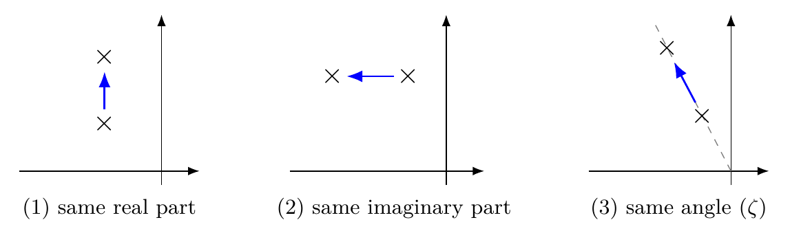
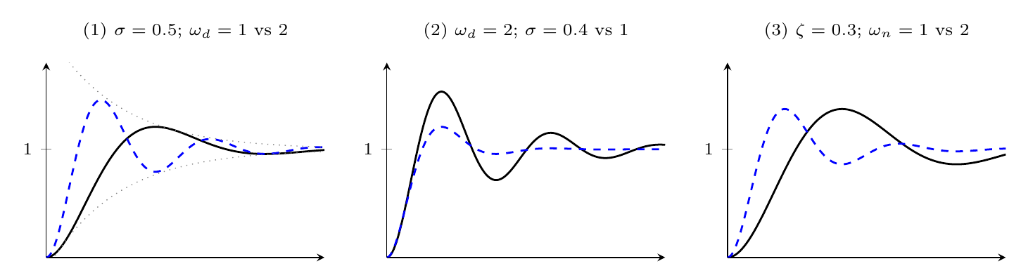
(1) Same real part, larger imaginary part. The envelope $e^{-\sigma t}$ is unchanged, so the responses settle within the same envelope, but the oscillation inside it is faster.
(2) Same imaginary part, further left. The oscillation frequency is unchanged, so the peaks occur at the same times, but the envelope decays faster and the response settles sooner.
(3) Same angle, further from the origin. The damping ratio $\zeta$ is unchanged, so the percentage overshoot is the same. The whole response is compressed in time: it rises, peaks and settles faster.
The responses confirm each prediction:
| Pole move | Envelope / $T_s$ | Oscillation / $T_p$ | $\%OS$ |
|---|---|---|---|
| (1) up, same real part | same | faster | increases |
| (2) left, same imaginary part | faster | same | decreases |
| (3) outward along a ray | faster | faster | same |
Summary and outlook
- The real part governs how fast the response settles, the imaginary part how fast it oscillates, and the angle how much it overshoots.
- An overshoot specification fixes a ray. Moving outward along that ray speeds everything up without changing the overshoot, which is exactly what the PD design of Lecture 17 will exploit.
The next lecture puts this intuition to work: it uses the root locus to design a PD controller that moves the closed-loop poles outward along the $\zeta$ line, speeding up the transient without changing the overshoot.
References
- N. S. Nise, Control Systems Engineering, 6th ed.: §4.6 Underdamped Second-Order Systems (p. 177).
- X. Chen and M. Tomizuka, Introduction to Modern Controls, with Illustrations in MATLAB and Python: §8.2.1 Method of Eigenvalue Locations (p. 144).