Lecture 17: Transient Design with Root Locus Using PD Control
Lectures 13–16 built up the root locus: how to sketch it (Lectures 13 and 14), how a fast pole limits the achievable gain (Lecture 15), and what each part of a pole location does to the response (Lecture 16). In this lecture we use the locus as a design tool. Lecture 7 tied the transient specifications to the location of a pair of complex poles, and Lecture 9 showed that a stable zero speeds up the response. Putting these together, we will see that adding a zero pulls the root locus to the left, which gives a faster transient at the same damping ratio. This is proportional–derivative (PD) design.
From specifications to pole locations
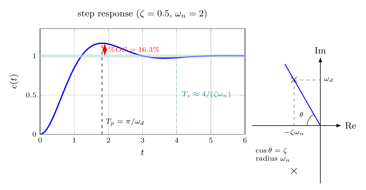
Recall the step response of the standard second-order system $\omega_n^2/(s^2 + 2\zeta\omega_ns + \omega_n^2)$ from Lecture 7. Its three transient specifications, the peak time $T_p$, the percent overshoot $\%OS$ and the settling time $T_s$, can be read directly from the plot, and each is tied to one feature of the pole location $s = -\zeta\omega_n \pm j\omega_d$:
| Quantity | Formula | Set by |
|---|---|---|
| Settling time | $T_s \approx 4/(\zeta\omega_n)$ | real part $-\zeta\omega_n$ |
| Peak time | $T_p = \pi/\omega_d$ | imaginary part $\omega_d$ |
| Overshoot | $\%OS = 100\,e^{-\zeta\pi/\sqrt{1-\zeta^2}}$ | angle $\theta$ only |
Let $\theta$ be the angle between the pole and the negative real axis. Then $\cos\theta = \zeta$. A target overshoot therefore fixes a ray from the origin, the $\zeta$ line. Design then reduces to deciding where on that ray the closed-loop pole should sit: further left means a smaller $T_s$, and further from the real axis means a smaller $T_p$.
The board example: P control on a three-pole plant
Consider unity feedback around the plant
$$G(s) = \frac{K}{(s+1)(s+2)(s+5)},$$with proportional control, so $K$ is the only design variable. We want $\zeta = 0.5$ (about $16\%$ overshoot).
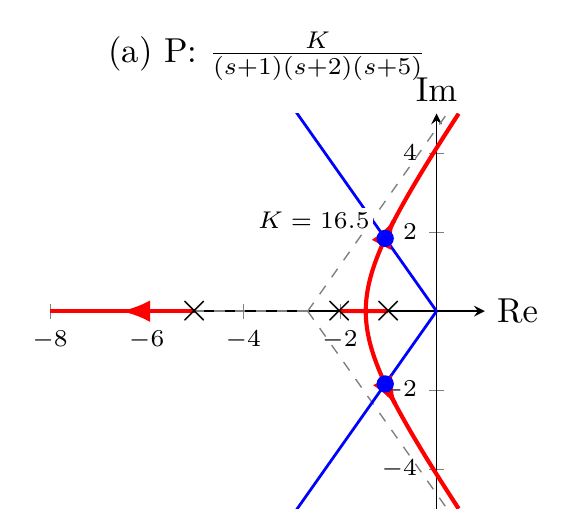
Sketching the locus. Three poles at $-1$, $-2$ and $-5$, no finite zeros.
- Real-axis segments: $[-2, -1]$ and $(-\infty, -5]$.
- Asymptotes: $n - m = 3$, at $\pm60^\circ$ and $180^\circ$, centered at $\sigma_a = (-1 - 2 - 5)/3 = -8/3$.
- The branch from $-5$ runs off to the left and is non-dominant. The branches from $-1$ and $-2$ meet, break away from the real axis and bend toward the $\pm60^\circ$ asymptotes.
Reading off the design. The $\zeta = 0.5$ line is the ray at $120^\circ$ from the positive real axis. The computed locus crosses it at
$$s = -1.06 \pm j1.84, \qquad K = |s+1|\,|s+2|\,|s+5| = 16.5,$$by the magnitude condition. The third closed-loop pole is at $-5.87$, about five times further left, so by Lecture 8 the pair at $-1.06\pm j1.84$ dominates. The predicted transient is
$$T_s = \frac{4}{1.06} = 3.8\ \text{s}, \qquad T_p = \frac{\pi}{1.84} = 1.7\ \text{s}, \qquad \%OS = 16\% .$$With P control there is nothing more to choose: the locus is fixed, and so is the point where it crosses the $\zeta$ line.
Adding a zero
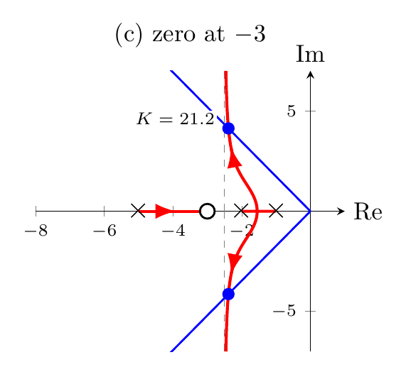
A zero changes the locus itself. Replace $K$ by a PD controller $K(s + z)$, which adds a zero at $-z$. The three loci below are all computed exactly: (a) P control, (b) a zero at $-2$, which cancels the pole there, and (c) a zero at $-3$. In each, the blue ray is the $\zeta = 0.5$ line and the dots are the resulting closed-loop poles.
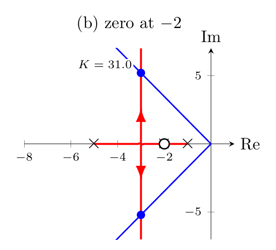
(b) Zero at $-2$. The loop becomes $K(s+2)/\big((s+1)(s+2)(s+5)\big) = K/\big((s+1)(s+5)\big)$. The effective poles are $-1$ and $-5$, so $n - m = 2$, the asymptotes are at $\pm90^\circ$, and the centroid is $(-1 - 5)/2 = -3$. The branches meet at $-3$ and go straight up and down. They cross the $\zeta$ line at
$$s = -3 \pm j5.20, \qquad K = 31.0 .$$(c) Zero at $-3$. Now $\sigma_a = \dfrac{(-1 - 2 - 5) - (-3)}{3 - 1} = -2.5$, again with $\pm90^\circ$ asymptotes. The branch from $-5$ moves right to the zero at $-3$, and the dominant pair crosses the $\zeta$ line at
$$s = -2.39 \pm j4.13, \qquad K = 21.2,$$with the third pole at $-3.23$, close to the zero at $-3$ (so its effect nearly cancels).
What moving the locus left buys us. At the same $\zeta$ line:
| Design | Dominant poles | $T_s = 4/(\zeta\omega_n)$ | $T_p = \pi/\omega_d$ |
|---|---|---|---|
| (a) P | $-1.06\pm j1.84$ | 3.8 s | 1.71 s |
| (b) zero at $-2$ | $-3.00\pm j5.20$ | 1.3 s | 0.60 s |
| (c) zero at $-3$ | $-2.39\pm j4.13$ | 1.7 s | 0.76 s |
- the closed-loop pole moves left, so $\zeta\omega_n$ increases and $T_s$ decreases;
- $\omega_d$ increases, so $T_p$ decreases;
- $\zeta$ is unchanged, so $\%OS$ is (nearly) unchanged.
The simulated step responses confirm the prediction: (b) and (c) are about three times faster than (a) with similar overshoot. (All three settle below 1: this type-0 loop has a steady-state error, the topic of Lecture 12 and of the lag compensator in Lecture 18.)
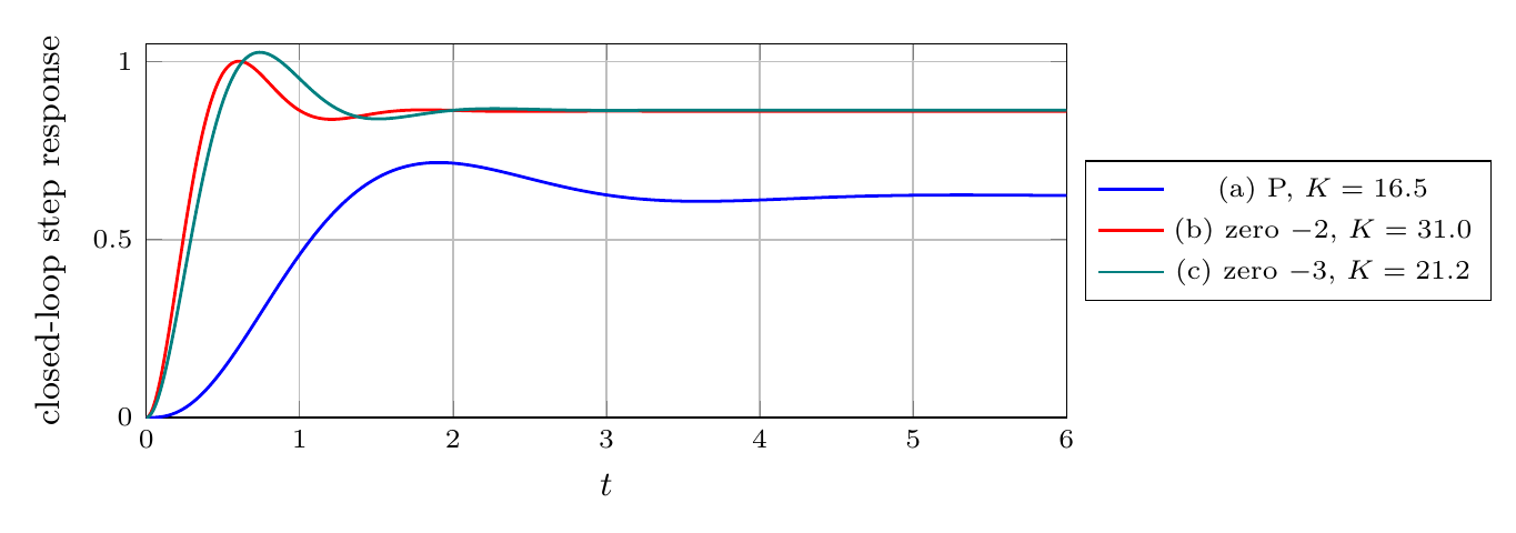
We get a faster transient with the same overshoot. The reason, from Lecture 9, is that a zero adds a derivative: while the signal rises, its derivative is positive and the rise is accelerated. Because the added factor $K(s+z) = Kz + Ks$ is proportional plus derivative, this is called PD control.
A complete design
We now carry out a full design with a specification on both overshoot and speed. The plant is
$$G(s) = \frac{K}{s(s+4)(s+6)},$$and we require $\%OS \le 16\%$ together with a settling time several times shorter than the uncompensated design. The lecture posed a $4\times$ reduction; the lecture notes (and Nise, Example 9.3) use $3\times$. We work both.
Step 1: the $\zeta$ line. From Lecture 7, $\zeta = \dfrac{-\ln 0.16}{\sqrt{\pi^2 + \ln^2 0.16}} = 0.504$. This is a ray at $180^\circ - \cos^{-1}\zeta = 120.26^\circ$ from the positive real axis.
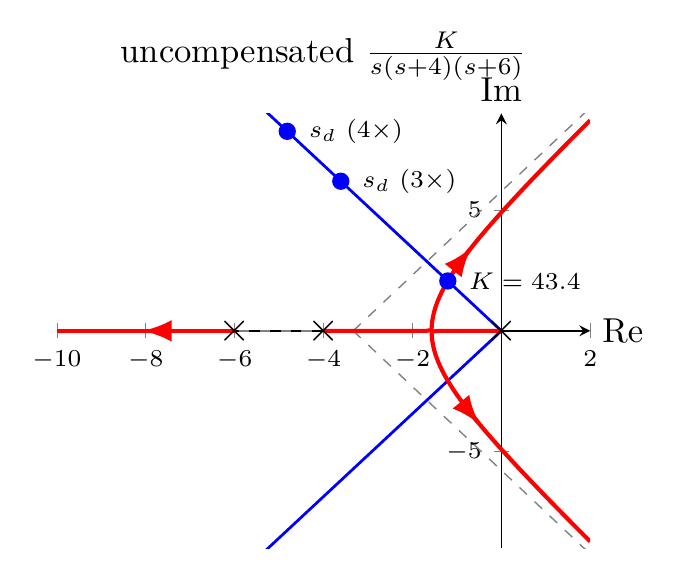
Step 2: the uncompensated design. The locus has centroid $(0 - 4 - 6)/3 = -10/3$ and asymptotes at $\pm60^\circ$ and $180^\circ$. The computed locus meets the $\zeta$ line at $s = -1.204 \pm j2.065$ with $K = 43.4$, so
$$T_s = \frac{4}{1.204} = 3.32\ \text{s}.$$Step 3: the target pole. To keep the overshoot, the new pole must stay on the same ray. To cut the settling time by the chosen factor, its real part must grow by that factor, which scales the whole pole along the ray:
| Speed-up | Target $T_s$ | Target pole $s_d$ |
|---|---|---|
| $3\times$ | $1.11$ s | $-3.61 + j6.19$ |
| $4\times$ | $0.83$ s | $-4.82 + j8.26$ |
The two targets are marked on the uncompensated locus below. Neither lies on it, so no gain alone can reach them.
Step 4: place the zero. We add a zero that bends the locus through $s_d$. For $s_d$ to lie on the new locus, $\angle\big((s_d + z_c)/(s_d(s_d+4)(s_d+6))\big) = \pm180^\circ$: the angle from the zero minus the angles from the three poles,
$$\alpha_1 - (\theta_1 + \theta_2 + \theta_3) = \pm180^\circ .$$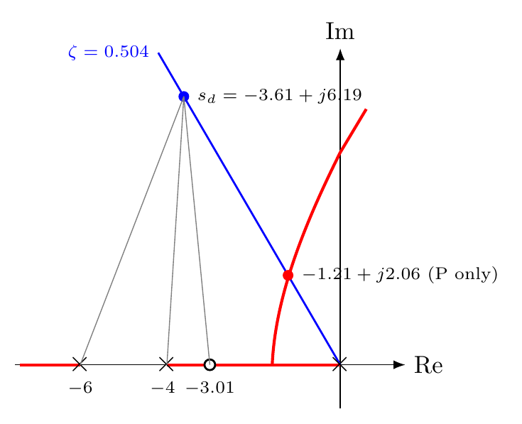
For the $3\times$ case, the angles from the poles at $0$, $-4$ and $-6$ to $s_d = -3.61 + j6.19$ are $\theta_1 = 120.26^\circ$, $\theta_2 = 86.42^\circ$ and $\theta_3 = 68.92^\circ$ (sum $275.60^\circ$), so the zero must contribute $\alpha_1 = 275.60^\circ - 180^\circ = 95.60^\circ$. Since this exceeds $90^\circ$, the zero lies slightly to the right of $s_d$:
$$z_c = 3.61 - \frac{6.19}{\tan(180^\circ - 95.60^\circ)} = 3.61 - 0.61 = 3.01,$$giving $C(s) = K(s + 3.01)$. The magnitude condition then gives $K = \dfrac{|s_d|\,|s_d+4|\,|s_d+6|}{|s_d+3.01|} = 47.5$. The same steps for the $4\times$ target give:
| Speed-up | Zero angle | PD zero | Gain $K$ | Third closed-loop pole |
|---|---|---|---|---|
| $3\times$ | $95.6^\circ$ | $-3.01$ | $47.5$ | $-2.77$ |
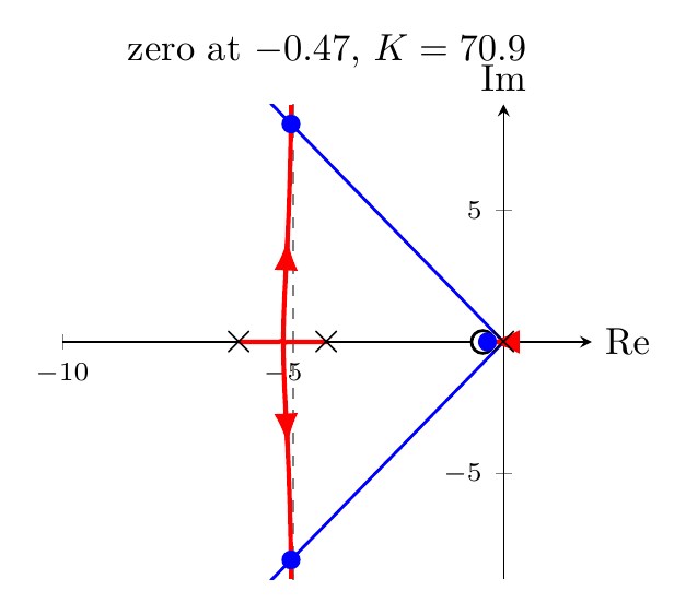
| $4\times$ | $117.8^\circ$ | $-0.47$ | $70.9$ | $-0.37$ |
The compensated loci pass exactly through the targets:
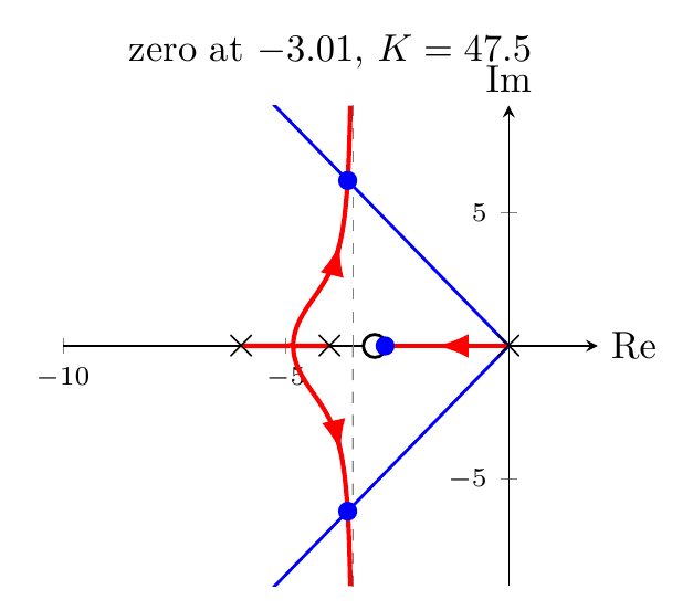
Step 5: check by simulation. In both designs the third closed-loop pole sits near the added zero, which suggests the second-order approximation holds. Simulation shows that this is true for the $3\times$ design but only partly true for the $4\times$ design:
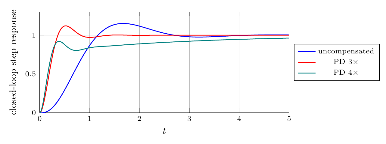
- $3\times$: overshoot $12\%$, $T_s = 1.16$ s, as designed. The pole-zero pair at $-2.77$/$-3.01$ nearly cancels.
- $4\times$: the fast dominant poles produce a quick initial rise, but the pair at $-0.37$/$-0.47$ is very slow (time constant $1/0.37 = 2.7$ s). The cancellation is not exact, so a small, slow tail remains and the 2% settling time stretches to about $6.7$ s.
The lesson is general: a near-cancelling pole-zero pair is harmless when it is fast, but a slow pair leaves a long tail even when its residue is small. Lecture 22 returns to this effect. Always confirm a root-locus design by simulation.
As a question for reflection: to obtain less than $16\%$ overshoot, should the $\zeta$ line rotate toward or away from the real axis?
Summary and outlook
- An overshoot specification fixes a $\zeta$ line; a $T_s$ or $T_p$ specification fixes the point on it.
- With P control, the design point is wherever the fixed locus crosses the $\zeta$ line.
- Stable zeros (PD control) pull the locus left, giving a faster transient at the same overshoot.
- Place the compensator zero with the angle condition, then find the gain from the magnitude condition, then simulate.
PD control improves the transient, but it does nothing for the steady-state error, and an ideal derivative amplifies noise. The next lecture replaces the ideal PD by its practical form, the lead compensator, and adds a lag compensator to improve the steady-state error.
References
- N. S. Nise, Control Systems Engineering, 6th ed.: §4.6 Underdamped Second-Order Systems (p. 177); §8.7 Transient Response Design via Gain Adjustment (p. 415); §9.1 Introduction (p. 456); §9.3 Improving Transient Response via Cascade Compensation (p. 469), including Example 9.3.
- X. Chen and M. Tomizuka, Introduction to Modern Controls, with Illustrations in MATLAB and Python: §8.2.1 Method of Eigenvalue Locations (p. 144).