Lecture 18: From PD Control to Lead Compensator and Steady-State Error Improvement with Lag Compensator
We now have tools to shape the transient (PD control, Lecture 17) and a way to measure steady-state accuracy (Lecture 12). This lecture connects the two sides. It first places the root-locus compensators in one framework, lead and lag, and then shows exactly how a lag compensator reduces the steady-state error, ending with a complete numerical design.
Lead and lag: practical PD and PI
The two ideal controllers of classical control each have a practical approximation:
| Ideal | Practical approximation | Improves | Pole–zero placement |
|---|---|---|---|
| PD: $K(s+z)$ | lead: $K\dfrac{s+z_c}{s+p_c}$ | transient | $\lvert z_c\rvert \lt \lvert p_c\rvert$ (pole further left) |
| PI: $K\dfrac{s+z}{s}$ | lag: $K\dfrac{s+z_c}{s+p_c}$ | steady state | $\lvert z_c\rvert \gt \lvert p_c\rvert$ (pole near origin) |
Why approximate? A pure derivative needs an active circuit and is costly, so a lead compensator adds a pole far to the left, which makes it realizable while keeping most of the zero’s effect. A pure integrator is also costly, so a lag compensator moves the pole slightly off the origin.
The names describe phase. At a point $s$ on the locus, the compensator contributes phase $\theta_z - \theta_p$, the angle from its zero minus the angle from its pole:
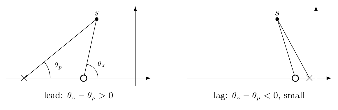
With the pole further left than the zero, $\theta_z \gt \theta_p$ and the compensator adds phase: it leads. With the zero further left, the contribution is negative, though small: it lags. A PI controller, with its pole exactly at the origin, raises the system type by one and, by Lecture 12, improves the steady state. The lag compensator approximates that effect.
How a lag compensator reduces the error
Extending Lecture 12 to a loop with controller $C$ and plant $G$, the error is $E = R/(1 + GC)$. If the closed loop is stable,
$$e_{ss}^{\text{step}} = \frac{1}{1 + \lim_{s\to0} G(s)C(s)},\quad e_{ss}^{\text{ramp}} = \frac{1}{\lim_{s\to0} sG(s)C(s)},\quad e_{ss}^{\text{parabola}} = \frac{1}{\lim_{s\to0} s^2G(s)C(s)}.$$In each case only the DC value of the compensator matters. For $C(s) = K\dfrac{s+z_c}{s+p_c}$,
$$C(0) = K\,\frac{z_c}{p_c},\qquad \frac{z_c}{p_c} \gt 1,$$since the pole and zero are both real and negative and the zero lies further left. The lag therefore multiplies the loop’s DC gain by $z_c/p_c \gt 1$. The denominator of $e_{ss}$ grows, so $e_{ss}$ shrinks. Placing the pair close to the origin keeps the transient nearly unchanged; Lecture 22 explains why.
The mechanism is the same for every input type. For a ramp input and the type-1 plant $G(s) = \dfrac{1}{s(s+1)(s+2)}$, $e_{ss} = \dfrac{1}{\lim_{s\to0}\frac{C(s)}{(s+1)(s+2)}} = \dfrac{2}{C(0)}$, and again a larger $C(0)$ means a smaller error. The parabolic case is left as an exercise.
A complete design
We now put these ideas to work on the plant
$$G(s) = \frac{1}{(s+1)(s+3)}.$$The design has two parts: first find the proportional gain $K$ that gives a closed-loop damping ratio $\zeta = 0.5$; then add a lag compensator that reduces the unit-step steady-state error by a factor of ten.
Part 1: the proportional design. The root locus of $KG$ has branches that meet at the centroid $-2$ and go vertically:
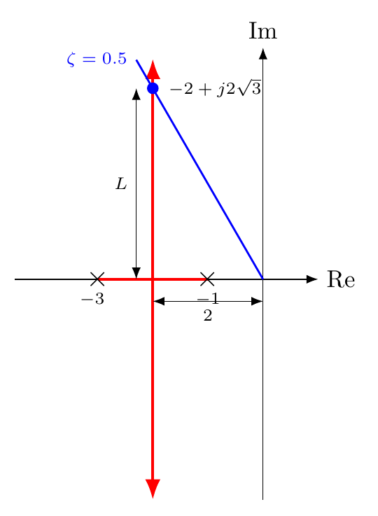
The desired pole lies where the $\zeta = 0.5$ line crosses the vertical branch. With $\tan\alpha = \sqrt{1-\zeta^2}/\zeta$ and a horizontal distance of $2$ from the origin,
$$\frac{L}{2} = \frac{\sqrt{1 - 0.25}}{0.5} = \sqrt3 \;\Longrightarrow\; L = 2\sqrt3,\qquad s_{1,2} = -2 \pm j2\sqrt3.$$The gain follows from matching characteristic polynomials:
$$(s+1)(s+3) + K = s^2 + 4s + 3 + K \overset{!}{=} (s+2)^2 + 12 = s^2 + 4s + 16 \;\Longrightarrow\; K = 13.$$The plant is type 0 with $G(0) = 1/3$, so the steady-state error to a unit step is
$$e_{ss} = \frac{1}{1 + K\,G(0)} = \frac{1}{1 + 13/3} = \frac{3}{16}.$$Part 2: the lag design. The target is $\tilde e_{ss} = 3/160$. If the lag compensator is used alone, with unit gain,
$$\frac{1}{1 + \frac{z_c}{p_c}\cdot\frac13} = \frac{3}{160} \;\Longrightarrow\; \frac{z_c}{p_c} = 3\left(\frac{160}{3} - 1\right) = 157,$$which is a very aggressive ratio. If instead we keep the proportional gain $K = 13$ and add the lag on top,
$$\frac{1}{1 + 13\cdot\frac{z_c}{p_c}\cdot\frac13} = \frac{3}{160} \;\Longrightarrow\; \frac{z_c}{p_c} = \frac{157}{13} \approx 12.08.$$Keeping the proportional gain relaxes the requirement considerably. Placing the pole near the origin, $p_c = 0.01$, gives:
| Design | $z_c/p_c$ | $z_c$ | Compensator |
|---|---|---|---|
| lag only | $157$ | $1.57$ | $\dfrac{s+1.57}{s+0.01}$ |
| $K = 13$ plus lag | $12.08$ | $0.1208$ | $13\,\dfrac{s+0.1208}{s+0.01}$ |
A quick check confirms the second design: $1/(1 + 13\cdot12.08/3) = 0.01875 = 3/160$.
Summary and outlook
- Lead and lag compensators are realizable versions of PD and PI: lead improves the transient, lag the steady state.
- A lag compensator scales the loop’s DC gain by $z_c/p_c \gt 1$, which reduces the steady-state error for step, ramp and parabolic inputs alike.
- Keep the proportional gain, add the lag on top, and place the pole–zero pair near the origin.
The next lecture combines both kinds of compensation in a complete PID design, carried out both by hand and in Python.
References
- N. S. Nise, Control Systems Engineering, 6th ed.: §9.2 Improving Steady-State Error via Cascade Compensation (p. 459); §9.3 Improving Transient Response via Cascade Compensation (p. 469); §9.4 Improving Steady-State Error and Transient Response (p. 482); §9.6 Physical Realization of Compensation (p. 503).