Lecture 22: Bode Plots: Dominant Poles, Zeros and Model Approximation

Scheduled release: week of November 16, 2026.

Download lecture notes (PDF)

Introduction

A transfer function describes both the modes that can appear in a response and the weight with which those modes are excited and observed. This distinction matters when reducing a model or interpreting a controller design. We begin with a PD-plus-lag feedback loop and examine when a nearby stable zero suppresses a slow mode. A matched exponential input then illustrates the role of a transfer-function zero more directly. Finally, a worked Bode example shows how the importance of a pole depends on the frequency band of interest.

PD plus lag compensation in the loop

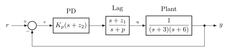
Consider a plant with poles at $-3$ and $-6$, controlled by a proportional-derivative (PD) factor and a lag factor. The additional controller pole makes the loop third order. Before deciding whether a second-order response approximation is reasonable, we must identify all of the closed-loop branches.

$$ G(s)=\frac{1}{(s+3)(s+6)},\qquad C(s)=K_p(s+z_2)\frac{s+z_1}{s+p}. $$

The loop $L=CG$ has three poles and two finite zeros, so the ordinary root locus has three branches and one branch going to infinity. Its asymptote angle is $180^\circ$, and its centroid is $-3-6-p+z_1+z_2$.

Root-locus branch count and asymptote

The branch count follows from the poles of the complete loop $L(s)=C(s)G(s)$, including the controller. The two finite zeros account for two branch endpoints; the remaining branch tends to infinity. This geometry identifies the possible closed-loop modes as the positive gain changes.

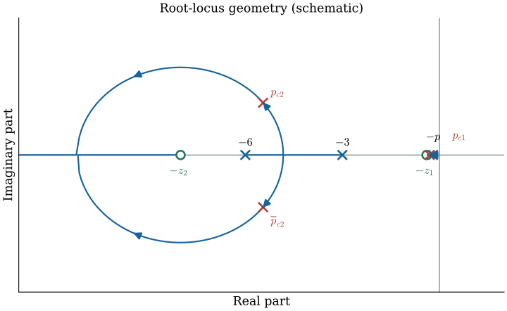
$$ \begin{aligned}n-m&=3-2=1,\\\sigma_a&=\frac{(-3)+(-6)+(-p)-(-z_1)-(-z_2)}{1}\\&=-9-p+z_1+z_2,\\\theta_a&=180^\circ.\end{aligned} $$

The root locus belongs to the complete loop $C(s)G(s)$. Its three branches begin at the three open-loop poles. Two branches terminate at the two finite zeros, while one goes to infinity along the negative-real direction. For any selected positive gain, there are three closed-loop poles, one on each branch. A slow real pole near the origin appears to challenge a second-order approximation based on the complex pair.

Dominant behavior depends on residues as well as poles

A root-locus plot locates the modes, but it does not by itself give their amplitudes in an input-output response. A slow pole may contribute little if a nearby numerator zero makes its residue small. We therefore examine the closed-loop transfer function as well as its characteristic roots.

$$ T(s)=\frac{K_p(s+z_1)(s+z_2)}{(s+p)(s+3)(s+6)+K_p(s+z_1)(s+z_2)}. $$

The numerator retains the finite open-loop zeros before cancellations. If a stable closed-loop pole is close to $-z_1$, that factor is approximately canceled and the complex pair may dominate the visible transient. This is an approximation, not an elimination of a state. For a simple pole $p_i$, the residue is $N(p_i)/D^{\prime}(p_i)$; a nearby numerator zero makes $N(p_i)$ small. A small slow term can still control the very late tail.

Factor the selected closed-loop poles

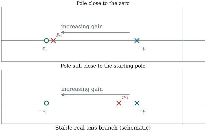
Factoring the denominator at the selected gain makes this suppression visible. The slow closed-loop pole and a nearby stable zero form a ratio that may be close to one over the frequency range of interest. The remaining factors then describe the dominant visible response.

$$ \begin{aligned}T(s)&=\frac{K_p(s+z_1)(s+z_2)}{(s-p_{c1})(s-p_{c2})(s-\overline{p}_{c2})},\\p_{c1}\approx-z_1&\ \Longrightarrow\ \frac{s+z_1}{s-p_{c1}}\approx1,\\T(s)&\approx\frac{K_p(s+z_2)}{(s-p_{c2})(s-\overline{p}_{c2})}.\end{aligned} $$

The finite zeros remain in the numerator after closing the loop. If the slow real closed-loop pole is near the lag zero, their ratio is close to one over the frequency range of interest. The complex pair can then dominate the visible response. The approximation is valid only when the selected gain places the pole sufficiently near the zero; it does not eliminate the corresponding internal state. A small residual slow mode can still affect the late tail.

When the approximation becomes inaccurate

The approximation depends on the actual closed-loop pole location, which changes with gain. An open-loop lag pole and zero being close is not sufficient on its own. Their effect must be assessed after the gain has been chosen and the resulting closed-loop roots are known.

$$ C_{\mathrm{lag}}(s)=\frac{s+z_1}{s+p},\qquad C_{\mathrm{lag}}(0)=\frac{z_1}{p},\qquad 0\lt p\lt z_1. $$

For a branch that ends at a finite zero, the selected gain determines how close its closed-loop pole is to that endpoint. Moving the lag pole and zero toward the origin while retaining their ratio can preserve the desired low-frequency gain and reduce their effect near a faster designed pair. Verify the actual time response rather than assuming exact cancellation. Never use an unstable pole-zero cancellation as a guarantee of internal stability; model error can expose the hidden unstable mode.

Move the lag pair while retaining its ratio

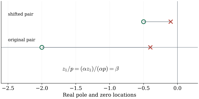
One way to reduce the lag pair’s influence on faster dynamics is to move both roots toward the origin while preserving their ratio. The ratio retains the DC gain improvement, whereas the smaller absolute root locations reduce their variation near the faster modes. This gives a useful design adjustment, subject to checking the resulting response.

$$ \begin{aligned}C_{\mathrm{lag}}(s)&=\frac{s+z_1}{s+p},\quad \beta=\frac{z_1}{p}\gt 1,\\\widetilde C_{\mathrm{lag}}(s)&=\frac{s+\alpha z_1}{s+\alpha p},\quad0\lt \alpha\lt 1,\\\widetilde C_{\mathrm{lag}}(0)&=\beta.\end{aligned} $$

The zero-to-pole ratio controls the low-frequency gain improvement. Scaling both locations toward the origin preserves that ratio while reducing their separation in absolute frequency. This can reduce disturbance of a faster designed complex pair. Low selected gain can still leave the real closed-loop pole near its starting pole rather than near the terminating zero, so inspect the actual response. Keep the pair stable; an unstable cancellation cannot certify internal stability.

A matched exponential input: the ODE

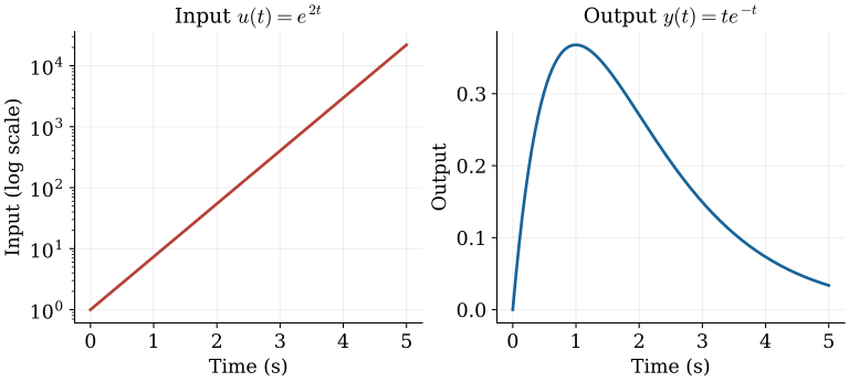
The preceding example concerns a zero reducing the contribution of a system mode. A different example shows that a zero can also suppress a specially matched input. Let $D$ denote differentiation with respect to time and consider a growing exponential whose exponent matches a right-half-plane zero.

$$ \begin{aligned}G(s)&=\frac{s-2}{s^2+2s+1},\quad u=e^{2t},\\\ddot y+2\dot y+y&=\dot u-2u,\\t\gt 0:\quad\dot u-2u&=2e^{2t}-2e^{2t}=0.\end{aligned} $$

The input grows without bound, but applying $D-2$ to $e^{2t}$ gives zero for $t\gt 0$. The output therefore obeys a homogeneous stable second-order equation, whose solutions are $(c_1+c_2t)e^{-t}$. They decay to zero. Initial conditions determine the constants. For a causal input switched on at zero, the switching event must be included; it supplies the initial derivative in the zero-state response.

The same example by Laplace transforms

The differential equation shows why the forcing vanishes for $t\gt 0$, but the causal switching condition still determines the response. A Laplace-transform calculation with zero initial state includes that switching automatically and identifies the remaining decaying output explicitly.

$$ \begin{aligned}U(s)&=\frac1{s-2},\\Y(s)&=\frac{s-2}{(s+1)^2}\frac1{s-2}=\frac1{(s+1)^2},\\y(t)&=te^{-t},\quad t\ge0.\end{aligned} $$

For zero initial state, the input transform has a pole exactly at the transfer-function zero. Their factors cancel in the product $G(s)U(s)$, leaving only stable output modes. The response has $y(0^+)=0$ and $\dot y(0^+)=1$, consistent with causal switching in the ODE. Any scalar multiple of this matched exponential has the same cancellation property. A different exponent would not cancel, so this is a signal-specific effect.

The separated-frequency worked example

We now return to frequency-response construction with a transfer function whose break frequencies are widely separated. This separation makes the contribution of each factor easy to follow. Normalizing the factors first exposes the DC gain and prevents a constant multiplier from being lost.

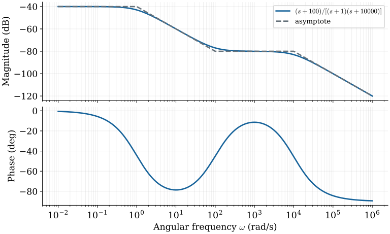
$$ G(s)=\frac{s+100}{(s+1)(s+10000)}=0.01\frac{1+s/100}{(1+s)(1+s/10000)}. $$

The DC gain is $0.01$, or $-40$ dB. The break frequencies are $1$, $100$, and $10000$ rad/s. Trace the accumulated magnitude slope through these locations: $0$, $-20$, $0$, then $-20$ dB/decade. The middle plateau is approximately $-80$ dB.

Build the magnitude one interval at a time

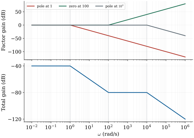
With the DC level and break frequencies identified, the magnitude sketch can be built continuously from left to right. Each new slope starts at the magnitude reached by the preceding interval. This preserves both the gain level and the accumulated effect of earlier factors.

$$ M(\omega)\approx\begin{cases}-40,&\omega\lt 1,\\-40-20\log_{10}\omega,&1\le\omega\lt 100,\\-80,&100\le\omega\lt 10^4,\\-80-20\log_{10}(\omega/10^4),&\omega\ge10^4.\end{cases} $$

The first pole lowers the slope by 20 dB/decade. Over the next two decades, the magnitude drops from $-40$ to $-80$ dB. The zero at 100 rad/s restores 20 dB/decade, giving a plateau. The pole at $10^4$ rad/s lowers the slope again. The exact curve rounds the corners, but its distant limits follow these lines. Every interval begins at the value reached by the preceding interval.

Dominance depends on the frequency band

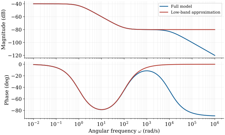
The separated breaks also clarify when a reduced model is useful. If the input frequencies are well below the fastest pole, that pole contributes almost a constant over the band of interest. Its dynamic variation may be neglected there, but its constant gain must remain in the approximation.

$$ \omega\ll10000:\qquad G(j\omega)\approx\frac{1}{10000}\frac{j\omega+100}{j\omega+1}. $$

For an input concentrated in a limited frequency band, evaluate the model in that band. The fast pole may be approximated by its DC factor, but cannot simply be deleted without rescaling. Remember that 10 Hz corresponds to about 62.83 rad/s. Omitted high-frequency modes can still matter for feedback robustness or broadband noise.

Add the three phase contributions

To complete the response, add the phase of the zero and subtract the phases of the two poles. Their separated locations produce distinct transitions. The final phase can also be checked from the relative degree: two poles and one zero give a net first-order high-frequency decay.

$$ \phi(\omega)=\tan^{-1}(\omega/100)-\tan^{-1}\omega-\tan^{-1}(\omega/10000). $$

The first pole ramps from $0.1$ to $10$ rad/s, the zero from $10$ to $1000$ rad/s, and the fast pole from $1000$ to $100000$ rad/s. The asymptotic phase therefore moves from $0$ to $-90^\circ$, back toward $0$, then toward $-90^\circ$. Use degrees/decade for phase slopes, not dB/decade. At high frequency the relative degree is one, which independently checks the $-90^\circ$ limit.

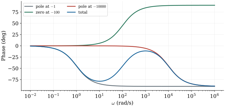
Mark each phase-ramp interval

The approximate phase curve follows by placing the two-decade transition interval around each break. In this example, the end of one ramp coincides with the beginning of the next. Adding their ordinates explains the recovery of phase between the two pole transitions.

$$ \begin{array}{c|c|c}\text{factor}&\text{transition interval (rad/s)}&\Delta\phi\\\hline1/(s+1)&0.1\ \text{to}\ 10&-90^\circ\\s+100&10\ \text{to}\ 1000&+90^\circ\\1/(s+10^4)&1000\ \text{to}\ 10^5&-90^\circ\end{array} $$

The first pole’s phase ramp ends at 10 rad/s just as the zero’s ramp begins. The zero then raises the total phase back toward zero before the final pole lowers it again. The accumulated asymptotic phase is $0\to-90^\circ\to0\to-90^\circ$. These are sums of the individual ordinates: a positive zero contribution must actually raise the total, not merely flatten an already completed pole transition.

Perspective

A useful approximation must preserve the behavior relevant to the input and frequency band under study. Pole locations determine decay rates, but zeros and residues determine how strongly those modes appear. Similarly, a distant pole may contribute almost no variation within a low-frequency band while still supplying an essential constant gain. The worked examples show why a reduced response should be checked against both the full transfer function and the intended operating conditions.

We next use the complete complex frequency response to address a different question: whether closing a feedback loop produces a stable system.

References

Norman S. Nise, Control Systems Engineering, 6th ed., Wiley, 2011.

• §§4.7–4.8: Additional poles, zeros, and dominant response.
• §§9.2–9.4: Cascade compensation.
• §10.2: Bode plots.