Lecture 1: The Power of Controls
Before we write a single transfer function, it is worth seeing why control engineering deserves a course of its own. This lecture takes three examples at very different scales: the human body, a semiconductor factory and a hard-disk drive. Each shows the same two ideas at work, feedback and feedforward, and together they show why modern technology depends on control. The second half of the lecture introduces the vocabulary used in the rest of the book: the elements of a control system, the objectives of control, and the path we will take to reach them.
Body temperature regulation
Our first example is one you are running right now. Your core body temperature stays near $98.6\,{}^\circ$F ($37\,{}^\circ$C) whether you are skiing on a snowy mountain or walking in a desert. If it drifts by a degree or two, you feel sick. How does the body hold such a steady value when the environment changes so much?
The answer is a feedback loop with a sensor, a controller and actuators. A small region at the back of the brain measures body temperature and compares it with the conditions outside. The skin then acts on that comparison. On a cold day, the muscles in the skin contract (your hair stands up), so less water reaches the surface and less heat is lost to evaporation. On a hot day, the muscles relax, the blood vessels dilate, more blood flows near the surface, and evaporation carries heat away faster. The brain keeps measuring, comparing and correcting.
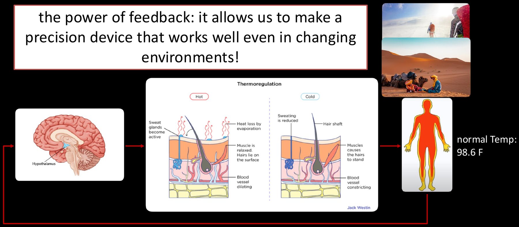
The power of feedback: it allows us to make a precision device that works well even in changing environments.
This is feedback, and it is remarkably robust: the loop keeps working even when you are slightly ill.
Humans add a second mechanism on top of this loop. Before going skiing, you check the forecast and put on more layers; on a hot day, you wear a T-shirt. Here you act on a prediction of the disturbance before it reaches your body. Acting on a measured or forecast disturbance in this way is called feedforward. Together, feedback and feedforward regulate body temperature to within one or two degrees Fahrenheit throughout the year and in complex environments.

Feedforward and prediction: acting before the disturbance arrives.
The two mechanisms can be drawn together as a block diagram. Block diagrams are the subject of Lecture 2; for now, read each box as something that acts on a signal.
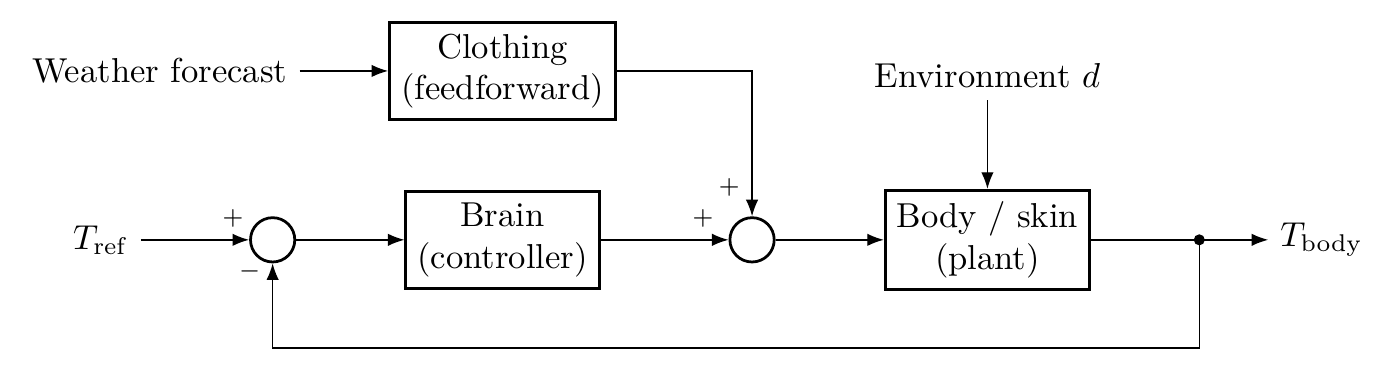
The same regulation loop can even be given a new purpose. Researchers have identified a brain “switch” that induces a hibernation-like state, controlled hypothermia, in animals that do not normally hibernate, by signalling the brain to lower body temperature and energy use (Current Biology, 2024). The loop is unchanged; only its target has moved. A control system, once understood, can be reconfigured to serve new goals.
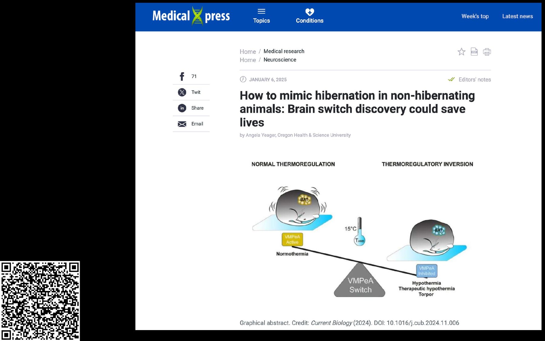
A brain “switch” for controlled hypothermia (Medical Xpress; graphical abstract from Current Biology, 2024).
Control in industry
The body shows the principle; industry shows the payoff. In large process plants, such as power generation or water treatment, advanced control is one of the technologies most often used to improve economic performance. The IEEE Control Systems Society report The Impact of Control Technology (2011) lists typical improvements:
| Improvement | Typical gain |
|---|---|
| Increased throughput | 3–5% |
| Reduced fuel consumption | 3–5% |
| Reduced emission levels | 3–5% |
| Reduced electricity consumption | 3–5% |
| Reduced quality variability | 10–20% |
| Reduced refractory consumption | 10–20% |
Because these plants are so large, a few percent of improvement can be worth millions of dollars.
Semiconductor manufacturing
Our second example moves to a much smaller scale. A modern GPU chip, such as the Blackwell-generation part shown at CES 2025, is roughly the size of a watch face yet holds about 92 billion transistors. They are “built” layer by layer by photolithography, in which light passes through a pattern and exposes features on a silicon wafer.
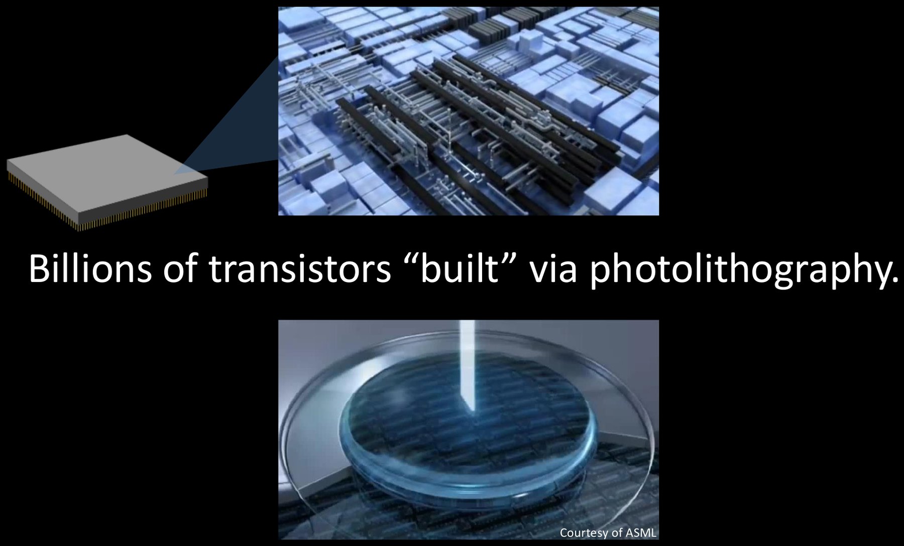
Billions of transistors built via photolithography (wafer image courtesy of ASML).
It is hard to picture a billion of anything. In stacked bills, USD 10,000 is a small stack and USD 1 million is about the size of a pair of shoes. USD 1 billion is a pile you could live in:
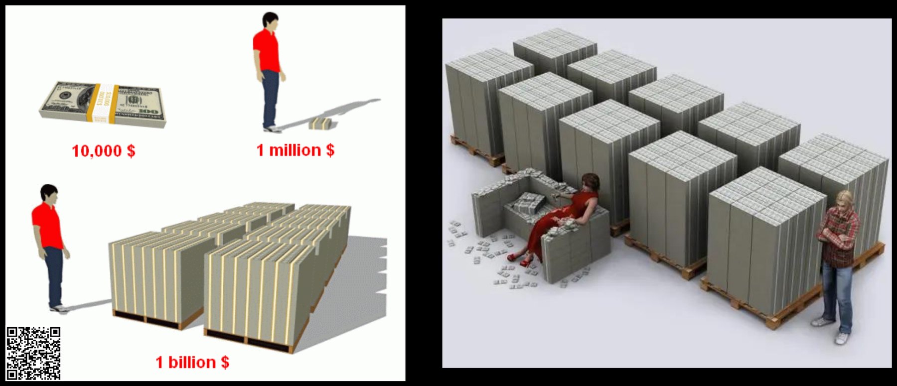
How big is a billion?
and in a picture of USD 1 trillion, a person is a speck in the corner:
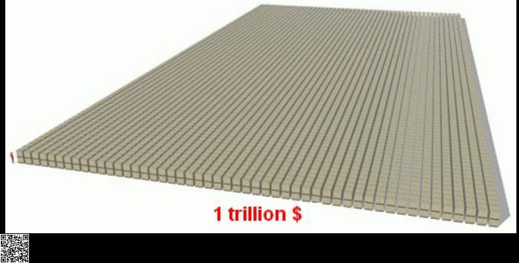
One trillion dollars, with a person for scale at the left corner.
No human could place parts at that count. The required precision is just as striking. Photolithography is nanometer-scale manufacturing. By analogy, it is like driving from Seattle airport (SEA) to campus (UW) 90 billion times, keeping every tire track within a millimeter of the last, at the same resolution every day, all year long.
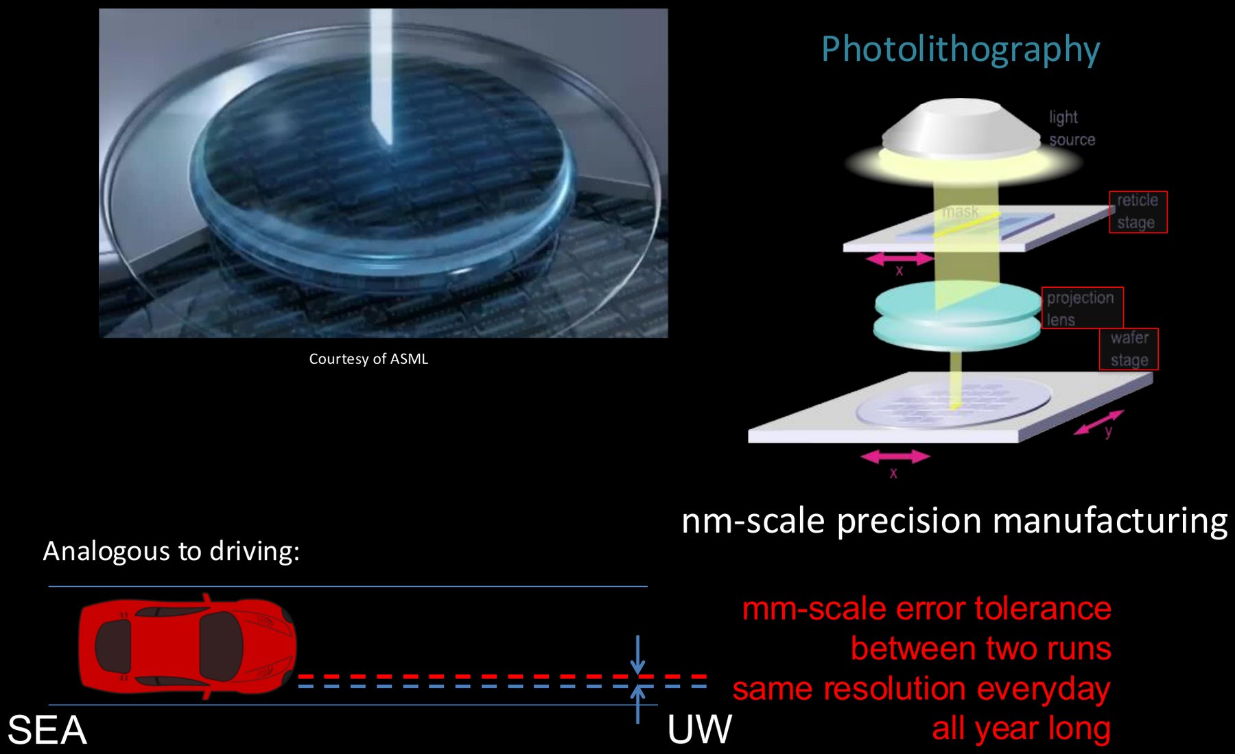
The control problem in photolithography and its driving analogy.
How can a machine reach such precision? One key observation is that lithography repeats the same motion over and over, so the errors repeat too, and a controller can learn them. With weak control the machine makes the same error on every run; with learning control the error shrinks from one iteration to the next:
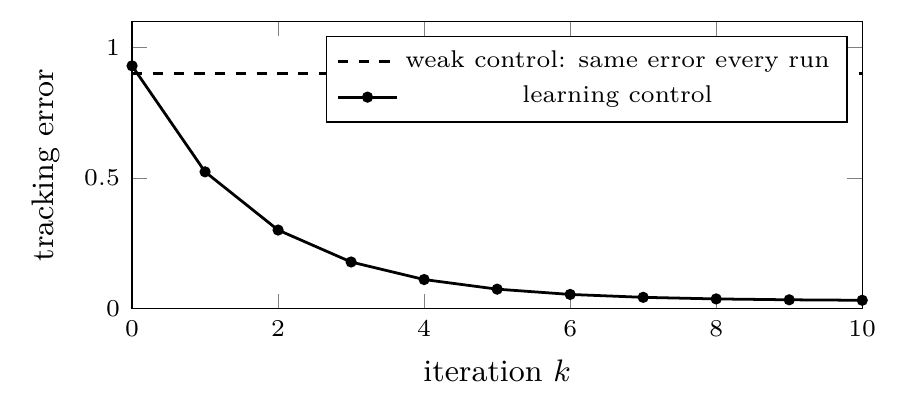
The curves above are illustrative. The measured position error of a wafer-scanning stage under weak control, on the order of $10^{-5}$ m, is shown below; enhanced control with feedback and prediction reduces it substantially.
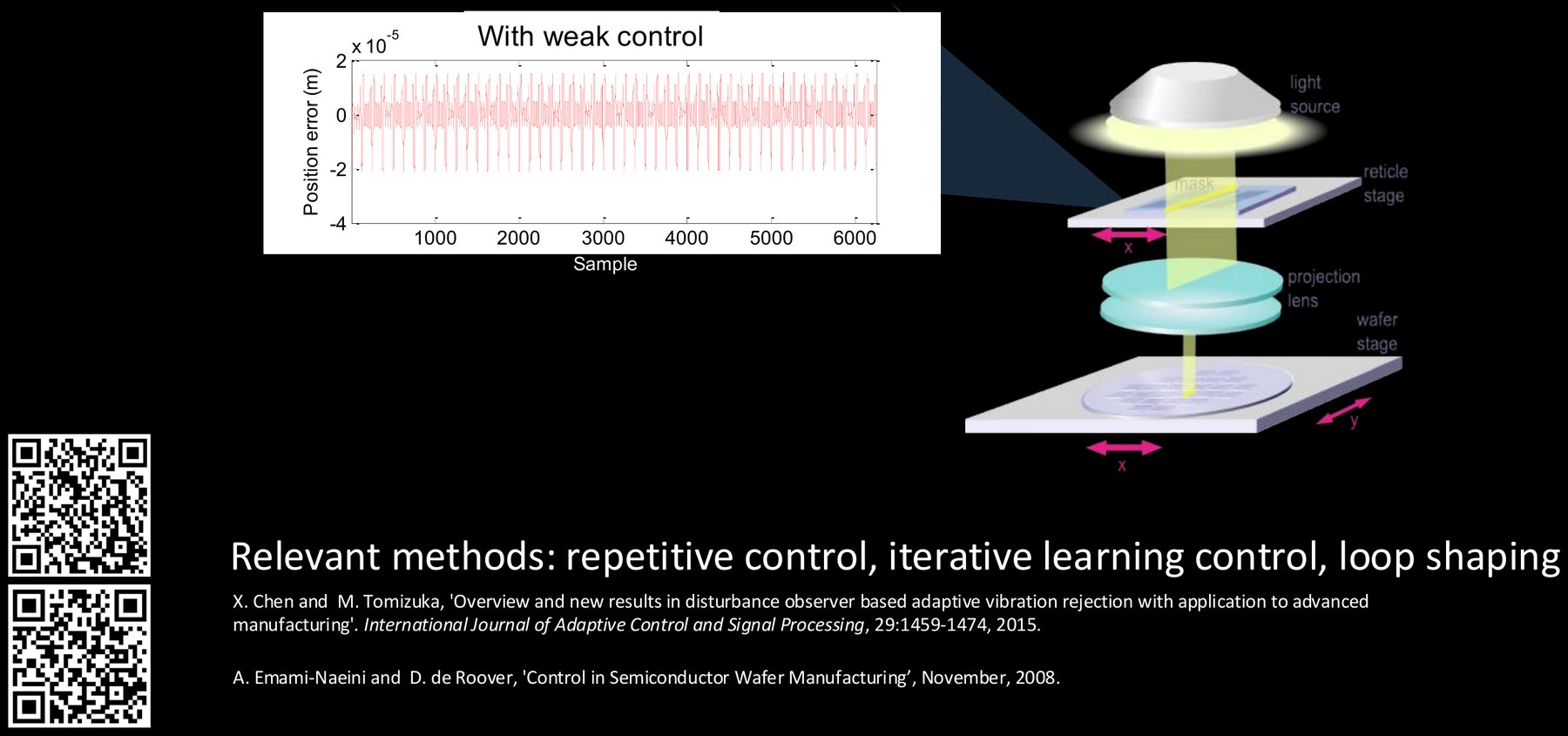
The power of feedback and prediction in wafer scanning.
The methods that make this possible, repetitive control, iterative learning control and loop shaping, are advanced topics, but they build on the foundations laid in this book. For more, see X. Chen and M. Tomizuka, “Overview and new results in disturbance observer based adaptive vibration rejection with application to advanced manufacturing,” International Journal of Adaptive Control and Signal Processing, 29:1459–1474, 2015; and A. Emami-Naeini and D. de Roover, “Control in Semiconductor Wafer Manufacturing,” 2008.
Hard-disk drives
Our third example is a device that is both extremely precise and extremely cheap. Inside an 8 TB hard drive, a read/write head on a rotary actuator moves above a spinning disk. It must follow data tracks with nanometer-scale precision and jump between tracks quickly.
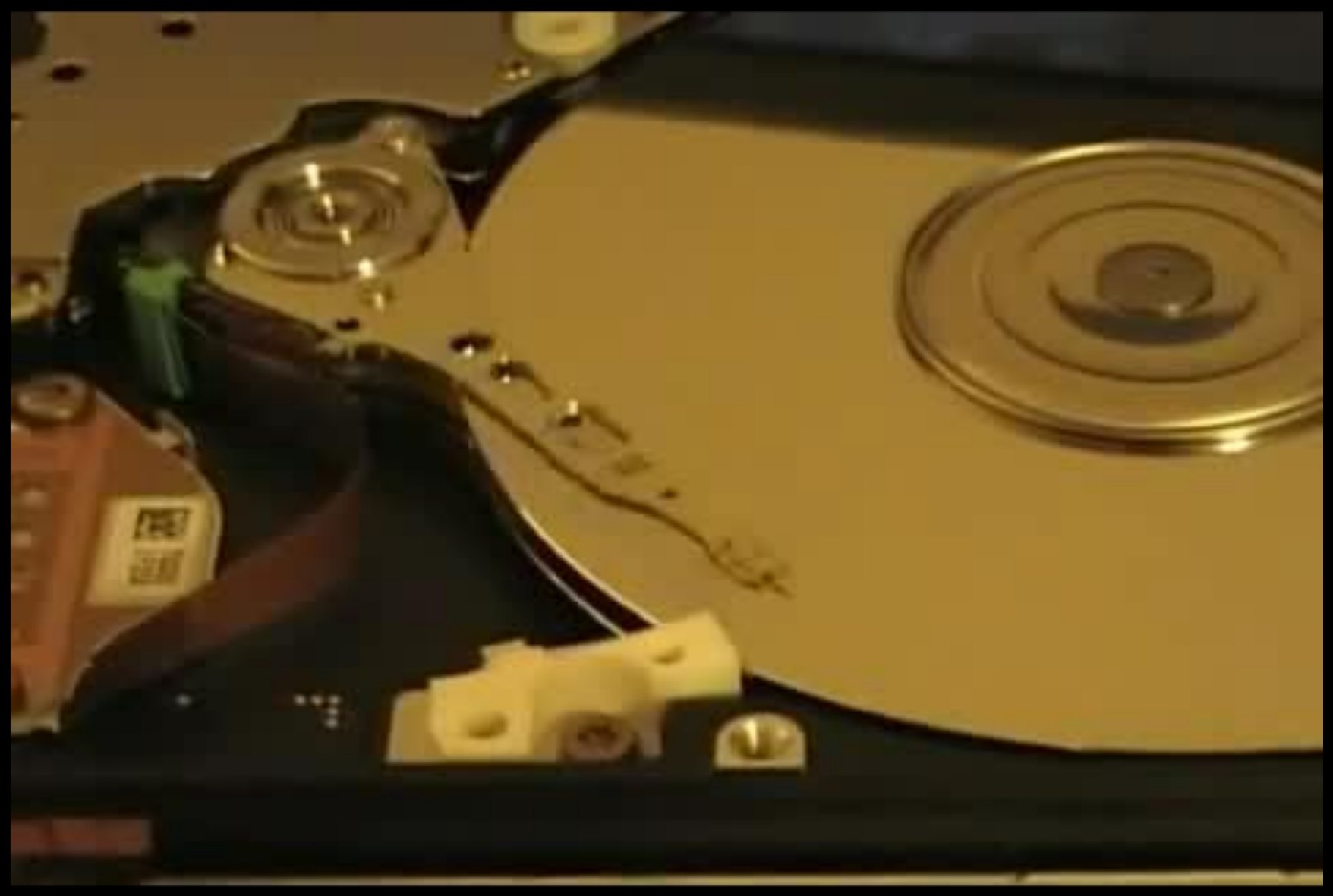
Inside a hard-disk drive.
A well-known analogy conveys the difficulty:
Imagine an airplane flying at 500,000 miles per hour but only 1/16 inch above the ground on a highway with 100,000 lanes where the width of each lane is only a fraction of an inch. The challenge of the problem is further intensified by the fact that the airplane is expected to switch lanes frequently and then follow the new lane with the same precision. A scaled-down version of this scenario is what one finds in the head positioning servomechanism of a hard disk drive.
— A. Al Mamun, G. Guo and C. Bi, Hard Disk Drive: Mechatronics and Control, 2007
A feedback loop solves this problem inside every disk drive.
Control everywhere
Control is everywhere. The IEEE Control Systems Society collects success stories in The Impact of Control Technology: mobile phones, flight control, pharmaceutical crystallization, unmanned aerial vehicles, wind energy capture, smart warehouses, automotive powertrains, power plants, Formula One, space launch, and many more.
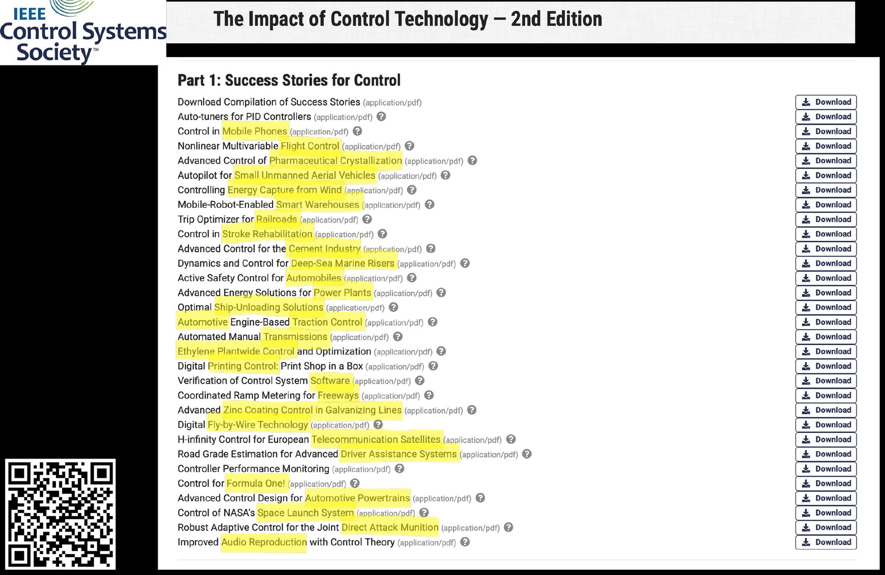
Success stories collected by the IEEE Control Systems Society.
More broadly, humans themselves are remarkable control systems. Returning a 230 km/h (143 mph) serve leaves no time for deliberate calculation; it relies on prediction and fast feedback between perception and the body.
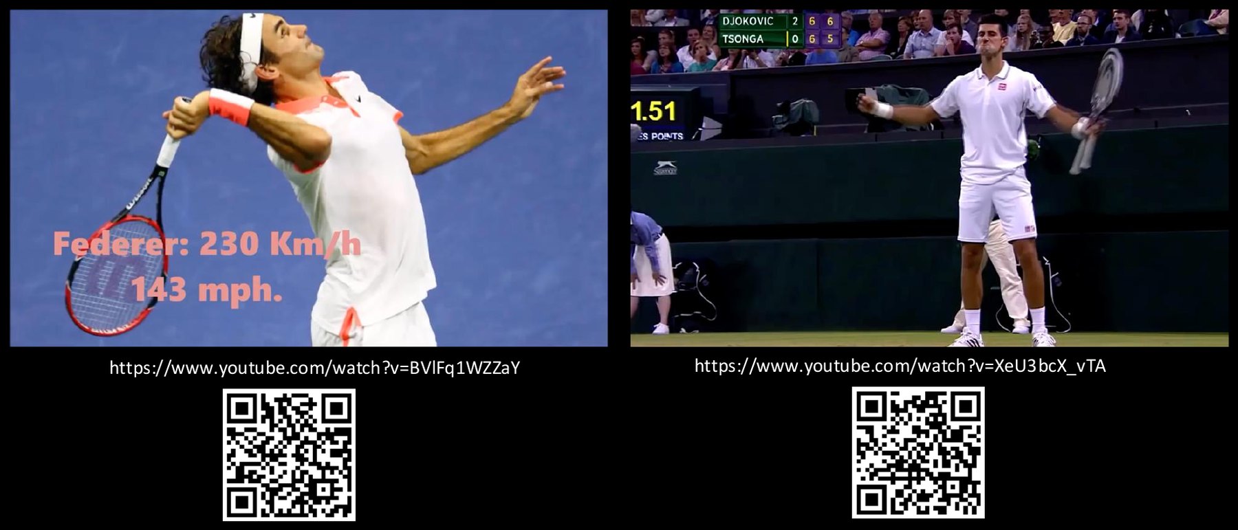
The mind–body–control nexus in elite tennis (videos: https://www.youtube.com/watch?v=BVlFq1WZZaY, https://www.youtube.com/watch?v=XeU3bcX_vTA).
Elements of a control system
The examples share a common structure, and naming its parts gives us a vocabulary for the rest of the book.
Dynamic systems. The systems we control are dynamic: they do not show the full effect of an input immediately, but only after a transient and/or a delay. Body temperature does not jump when you step into the cold; it adjusts over time, and it even follows a daily circadian rhythm. We describe inputs and outputs as signals, functions of time.
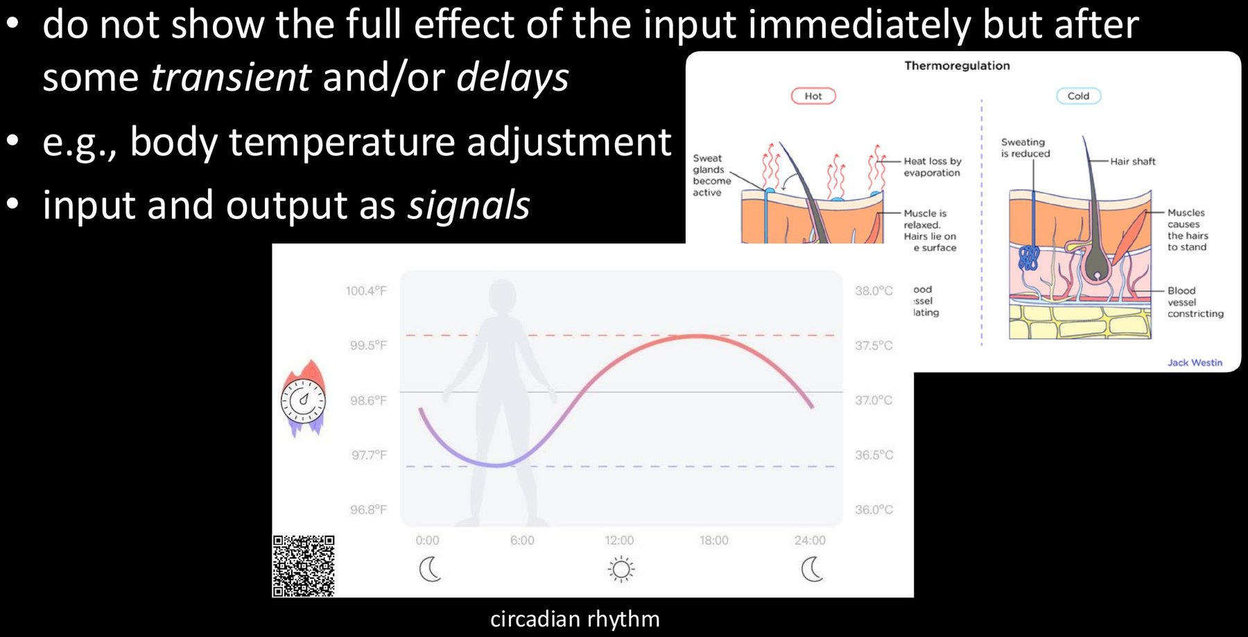
Dynamic systems: body temperature responds with transients and follows a circadian rhythm.
Process, actuator, plant and sensor. The process is what we ultimately want to control. The actuator is what acts on it, and together they form the plant. A sensor measures the output, inevitably adding sensor noise. The controller compares the measurement with the reference (possibly shaped first by an input filter) and commands the actuator. Disturbances enter at the process.
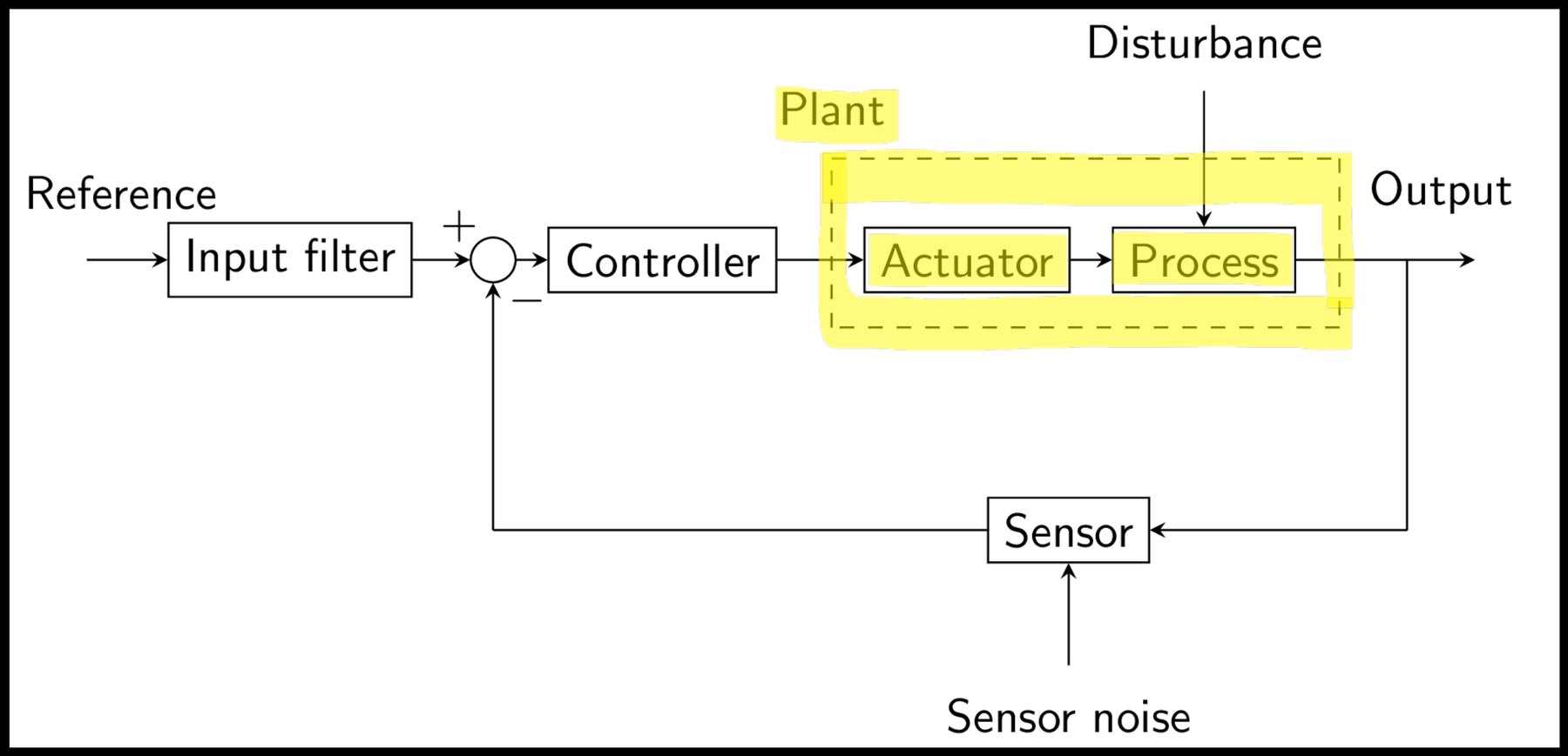
Process, actuator, plant, sensor and controller in a block diagram.
These elements appear in every example. In body temperature control, the brain is the controller, the skin is the actuator, the body is the process, and temperature sensing in the brain closes the loop. In automobile cruise control, the throttle and engine form the actuator, the auto body is the process, road grade is the disturbance, and the speedometer is the sensor.
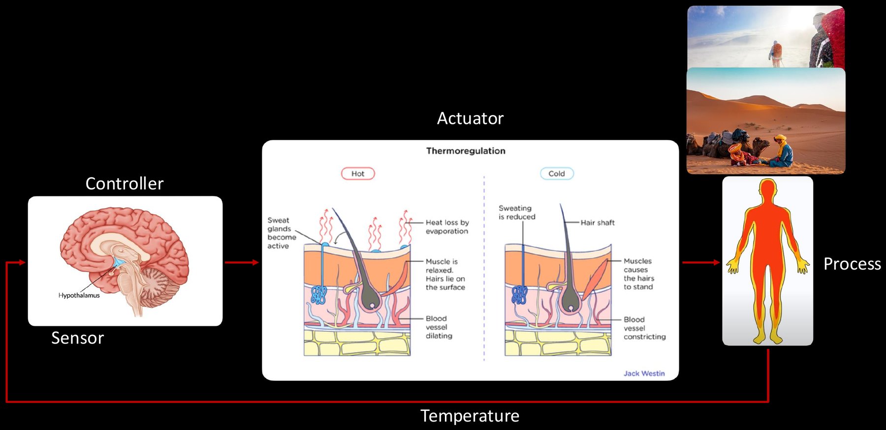
Body temperature control mapped to the block diagram.
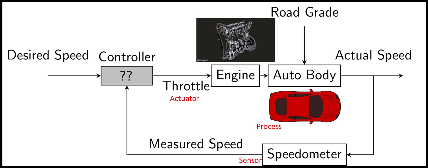
Automobile cruise control.
Open loop versus closed loop. An open-loop controller computes the input $u(t)$ from the desired output alone. It cannot see disturbances, so it cannot correct for them. In a closed-loop system, the components (plant, controller and so on) form a closed interconnection, so there is always feedback. A home thermostat is the classic example: it measures room temperature and adjusts the gas valve and furnace to counter heat loss.
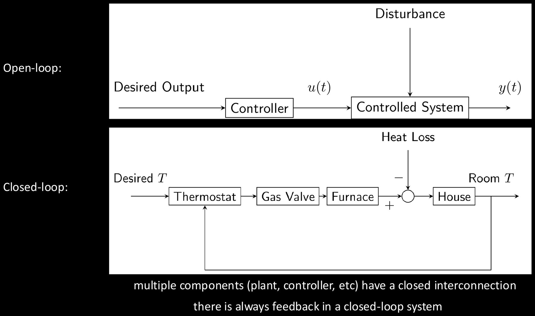
Open-loop control versus closed-loop control of room temperature.
Control objectives
What do we want a control system to achieve? Five objectives recur:
- Better stability.
- Improved response characteristics.
- Regulation of the output against disturbances and noise.
- Robustness to plant uncertainties.
- Tracking of a time-varying desired output.
Different applications emphasize different objectives. Body temperature regulation needs 1, 3 and 4; lithography needs 1, 2 and 5; hard-disk drives and athletes need all five; cruise control needs 1, 2, 3 and 4.
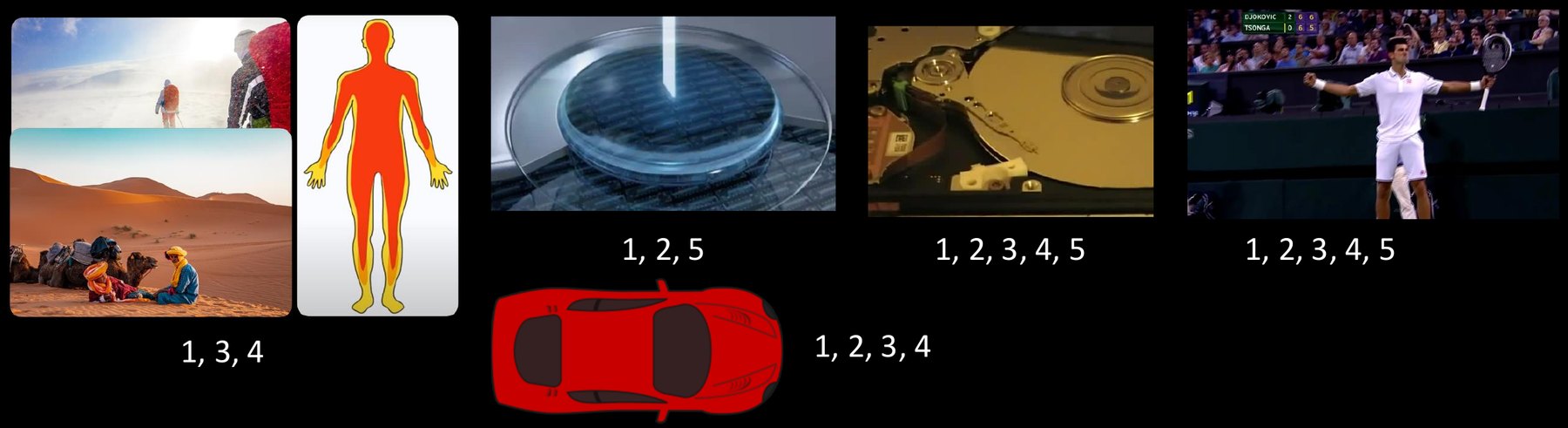
Which objectives matter in each example.
How we will get there
Meeting these objectives follows the same broad path in every application:
- Model the controlled plant.
- Analyze the characteristics of the plant.
- Design control algorithms (controllers).
- Analyze the performance and robustness of the control system.
- Implement the controller.
In classic control, the subject of this book, we describe systems with differential equations, the Laplace transform, transfer functions, block diagrams and frequency responses. We analyze their transient and steady-state behavior, stability, poles and zeros, and gain and phase margins. We design controllers with PID control, the root locus, lead-lag compensation and Bode/Nyquist loop shaping, with attention to sensitivity and robustness.
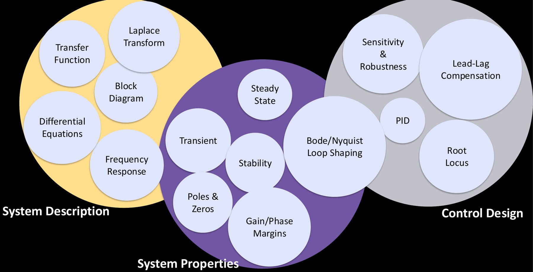
The landscape of classic control: system description, system properties and control design.
Modern control covers the same ground in state space: state-space models and their discretization and realization; properties such as stability, controllability and observability; and design methods such as state estimation, LQR, the Kalman filter and LQG.
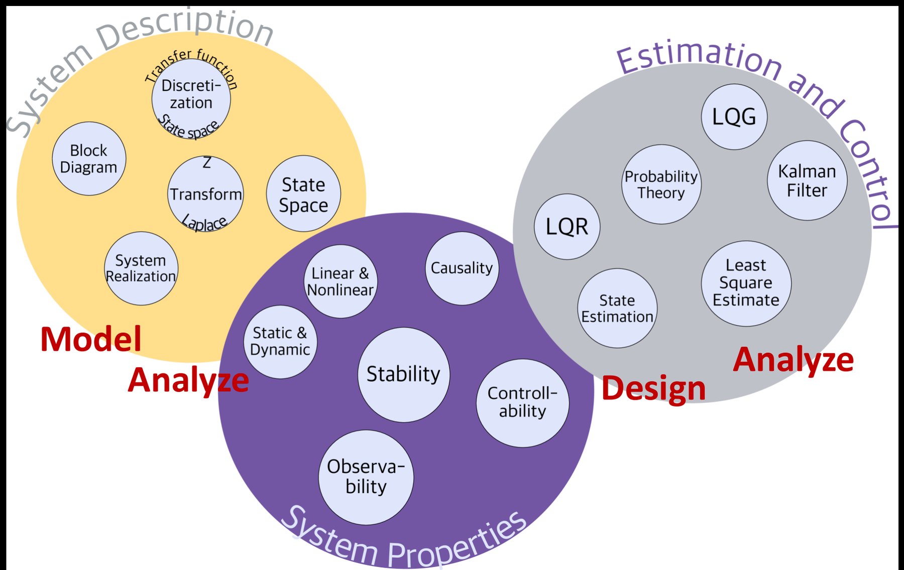
The landscape of modern control.
Beyond both lie more advanced topics that move from model-based toward data-driven methods: robust control, system identification, model predictive control (MPC), reinforcement learning, imitation learning, and large language and foundation models. For further reading, the IEEE Control Systems Society (in particular IEEE Control Systems Magazine), ASME (Journal of Dynamic Systems, Measurement and Control), AIAA and IFAC (Automatica, Control Engineering Practice) are good places to start. A standard classic-control textbook is N. S. Nise, Control Systems Engineering.
Summary and outlook
- Feedback measures the output, compares it with the goal and corrects, making a system precise and robust in an uncertain, changing environment.
- Feedforward uses prediction or measurement of disturbances to help the loop.
- Every control system consists of a controller, an actuator, a process and a sensor. Its objectives are stability, response, regulation, robustness and tracking.
- We reach those objectives by modeling, analysis, design and implementation.
The first step on that path is a language for describing how signals flow through interconnected components. That language is the transfer function and the block diagram, where Lecture 2 begins.
References
- N. S. Nise, Control Systems Engineering, 6th ed.: §1.1 Introduction (p. 2); §1.3 System Configurations (p. 7); §1.4 Analysis and Design Objectives (p. 10); §1.5 The Design Process (p. 15).
- X. Chen and M. Tomizuka, Introduction to Modern Controls, with Illustrations in MATLAB and Python: §1.1 The Power of Controls (p. 1); §1.2 Relevant Terminologies (p. 1); §1.3 The Objectives and The Means of Controls (p. 3); §1.4 Societies to Learn More about Controls (p. 5).