Lecture 24: Nyquist Stability: Encirclements and the Nyquist Criterion

Download lecture notes (PDF)

Introduction

The argument principle counts zeros and poles through a net change of phase. For negative feedback, applying it to $F(s)=1+L(s)$ counts the unstable roots of the closed-loop characteristic equation. The next step is to express that count in terms of the loop response $L(s)$ itself. This produces the Nyquist criterion: a signed encirclement count about $-1$, interpreted together with the unstable open-loop pole count. Throughout, counterclockwise image encirclements are positive and the domain contour is clockwise.

Why use frequency-domain stability analysis?

Direct root calculations establish stability for a particular model, but frequency-response geometry also helps explain how close a design is to losing stability. It can use a modeled or measured response, provided the open-loop unstable pole count and the assumptions of the stability test are available.

$$ L(j\omega)=|L(j\omega)|e^{j\phi(\omega)}. $$

Characteristic-root calculations and the Routh criterion test nominal stability. Practical models also have uncertainty: a flexible structure can reveal neglected modes at high frequency, and a motor model is never exact. Frequency-response geometry both tests stability and leads to gain and phase robustness margins. Frequency responses may also be measured experimentally from input and output sinusoids. The unstable open-loop pole count is still needed; the rational Nyquist argument here applies to LTI systems.

Signed turns about a reference point

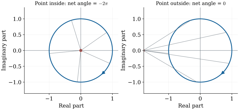
A geometric stability test first needs an unambiguous way to count turns. Choose a reference point and track the continuous angle of the ray from that point to the moving image. Local loops and changes of direction matter only through their signed net contribution over the complete traversal.

$$ \Delta\arg F=2\pi N_{\mathrm{CCW}},\qquad N_{\mathrm{CCW}}=N_{+}-N_{-}. $$

Track a ray from the chosen reference point to the moving point on the curve. An outside loop can move the ray back and forth without a complete turn. A clockwise turn contributes $-1$ and a counterclockwise turn contributes $+1$. Two clockwise turns give $-4\pi$ of unwrapped angle. Changing the reference point can change the count even when the curve is unchanged. The arrows, reference point, and full traversal are therefore all part of the calculation.

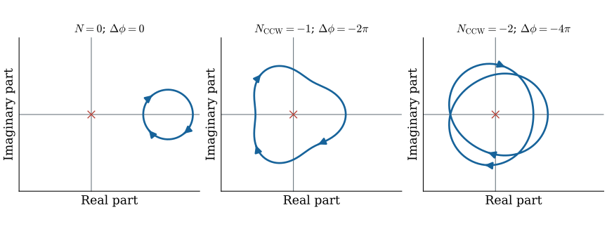
Net encirclements and the argument principle

This signed count gives a convenient unit for the argument principle: divide the net phase change by $2\pi$. With a clockwise domain contour and counterclockwise-positive image winding, the result is the number of enclosed poles minus the number of enclosed zeros.

$$ N_{\mathrm{CCW}}=\frac{\Delta\arg F}{2\pi}=P-Z. $$

The domain contour is traversed clockwise. The image curve can traverse either direction. Here counterclockwise image encirclements are positive, and clockwise encirclements are negative. An exterior reference point has zero winding even if the curve itself contains loops. A curve through the reference point has no well-defined winding number for this test.

The complete right-half-plane contour

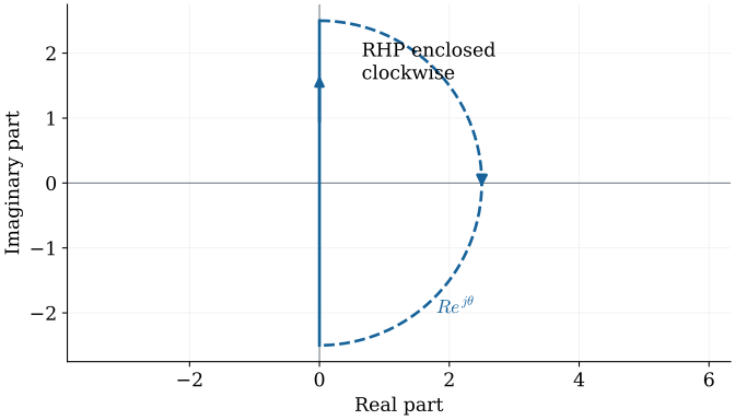
To count unstable roots, the domain contour must enclose the right half-plane. The ordinary Nyquist contour follows the imaginary axis and returns along a large semicircle. Initially, assume that no pole or characteristic root lies on this contour.

$$ s=j\omega\ (0\to R),\quad s=Re^{j\theta}\ (\pi/2\to-\pi/2),\quad s=j\omega\ (-R\to0). $$

For a strictly proper rational loop, $L(s)\to0$ on the large arc as $R\to\infty$. For a proper loop with nonzero direct term, use its actual finite limit. Do not assume this collapse for an improper loop. With real coefficients, $L(-j\omega)=\overline{L(j\omega)}$, so the negative-frequency branch is a reflection of the positive-frequency branch, with traversal order inherited from the contour.

Map the three contour segments

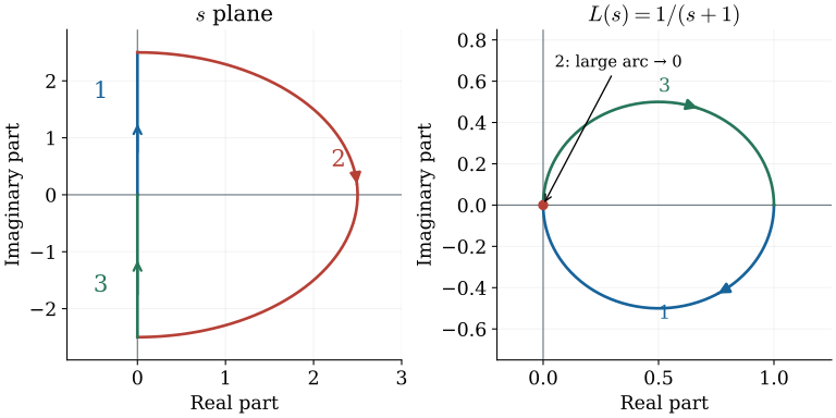
Each part of the domain contour contributes to the mapped curve. The positive-frequency response supplies one branch, the large semicircle supplies its high-frequency connection, and the negative-frequency response supplies the return branch. The traversal directions must remain consistent through all three segments.

$$ \begin{aligned}\Gamma_1:&\quad L(j\omega),\ \omega:0\to R,\\\Gamma_2:&\quad L(Re^{j\theta}),\\\Gamma_3:&\quad L(-j\omega)=\overline{L(j\omega)}.\end{aligned} $$

On the first segment, use the ordinary positive-frequency response. On the large semicircle, let $\theta$ decrease from $\pi/2$ to $-\pi/2$; a strictly proper transfer function tends uniformly to zero there. The third segment moves from $-jR$ to the origin, so the reflected frequency branch must be traversed in reverse frequency order. Increase $R$ enough to enclose every right-half-plane root before taking the limit.

The critical point is minus one

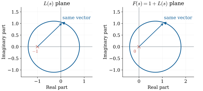
The argument principle applies to $F=1+L$, but the frequency response usually available is that of $L$. Adding one translates the entire image one unit to the right. We can therefore count turns of $L$ around $-1$ instead of turns of $F$ around the origin.

$$ Z=P-N_{\mathrm{CCW}},\qquad N_{\mathrm{CCW}}=\operatorname{wind}_{-1}\!L(\Gamma). $$

The closed loop is stable when $N_{\mathrm{CCW}}=P$ and no characteristic root lies on the imaginary axis. If the image passes through $-1$, then $1+L=0$ at a boundary point and the strict stability conclusion fails. The initial theorem assumes no open-loop pole lies on the imaginary axis; those poles require an indented contour.

Translate the origin to the critical point

This translation preserves more than the overall shape: it preserves the reference vector at every point. The vector from $-1$ to $L(s)$ is exactly $1+L(s)$. Its continuously tracked angle is therefore the same angle used in the argument-principle calculation.

$$ \begin{aligned}F(s)&=1+L(s),\\F(s)-0&=L(s)-(-1),\\\operatorname{wind}_{0}F&=\operatorname{wind}_{-1}L.\end{aligned} $$

For the same domain point, the vector from the origin to $F(s)$ is exactly the vector from $-1$ to $L(s)$. The vectors have the same length and angle throughout the traversal. We may therefore count turns about $-1$ on the loop curve instead of drawing $1+L$ separately. Combining this translation with the argument principle gives $N_{\mathrm{CCW}}=P-Z$.

Unstable first-order example

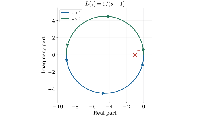
The criterion is particularly useful when the open loop is unstable. For $L(s)=9/(s-1)$, there is one right-half-plane pole, so stability requires one counterclockwise encirclement of $-1$. We can determine that count from an elementary circle.

$$ L(j\omega)=\frac{-9}{1+\omega^2}-j\frac{9\omega}{1+\omega^2},\qquad T(s)=\frac{9}{s+8}. $$

The positive-frequency curve starts at $-9$ and follows the lower semicircle toward the origin. Reflection supplies the upper half. The complete circle has center $-4.5$ and radius $4.5$, and encircles $-1$ once counterclockwise. Thus $P=1$, $N_{\mathrm{CCW}}=1$, and $Z=0$. Direct calculation gives the closed-loop pole $-8$, confirming the geometric result.

Construct the first-order Nyquist circle

To construct this circle rather than merely recognize its equation, calculate a few reference points and retain their frequency order. The zero-frequency value, the value at $\omega=1$, and the high-frequency limit anchor the positive branch. Conjugate symmetry then supplies the return branch.

$$ \begin{aligned}x&=\frac{-9}{1+\omega^2},\quad y=\frac{-9\omega}{1+\omega^2},\\(x+9/2)^2+y^2&=(9/2)^2.\end{aligned} $$

At $\omega=0$, the image is $-9$. At $\omega=1$, it is $-4.5-j4.5$. As positive frequency tends to infinity, the curve approaches zero from below with phase tending to $-90^\circ$. These points determine the lower semicircle; the negative frequencies complete the upper semicircle. The positive branch and the reflected return branch together travel counterclockwise around $-1$.

Stable first-order comparison

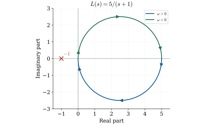
Now compare a stable first-order loop, $L(s)=5/(s+1)$. Here $P=0$, so the required encirclement count changes even though the image is again a circle. The different position of this circle illustrates why the pole count and the location of $-1$ must be considered together.

$$ L(j\omega)=\frac{5}{1+\omega^2}-j\frac{5\omega}{1+\omega^2},\qquad T(s)=\frac{5}{s+6}. $$

The curve starts at $+5$ and remains on the right-side circle. It does not encircle $-1$. Since $P=0$ and $N_{\mathrm{CCW}}=0$, the closed loop has no unstable roots. Its pole is $-6$. Numerical plotting should retain arrows and the conjugate branch; a plot without orientation is incomplete evidence for a signed count.

A higher-order loop can destabilize feedback

The stable first-order example does not imply that stable open-loop poles always yield stable feedback. Adding poles can supply enough phase lag for the Nyquist curve to surround $-1$ in the destabilizing direction. The loop $50/(s+1)^3$ provides a direct counterexample.

$$ (s+1)^3+50=0,\qquad s=-1+\sqrt[3]{50}\,e^{j(\pi+2k\pi)/3},\quad k=0,1,2. $$

The roots are approximately $-4.684$ and $0.842\pm j3.190$. Thus there are two unstable closed-loop roots. The complete Nyquist curve has net winding $N_{\mathrm{CCW}}=-2$ around $-1$, consistent with $P=0$ and $Z=2$.

Perspective

The criterion is $Z=P-N_{\mathrm{CCW}}$: the complete oriented curve supplies the signed encirclement count, and the open-loop model supplies $P$. The examples demonstrate both stabilization of an unstable open loop and destabilization of a stable one. If an open-loop pole lies on the imaginary axis, the ordinary contour cannot be used unchanged; its path must be indented before the argument-principle count is applied.

The next lecture develops the detours needed for poles on the imaginary axis and shows how to map their image arcs.

References

Norman S. Nise, Control Systems Engineering, 6th ed., Wiley, 2011.

• §§10.3–10.5: Nyquist criterion, diagrams, and stability.