Lecture 9: The Effect of Zeros
Lecture 8 studied how poles combine while keeping the numerator constant. We now complete the picture by adding a zero. Zeros do not create new modes, since the modes come from the poles, but they change how strongly each mode appears. The result is sometimes a faster rise and sometimes a response that starts in the wrong direction. This lecture explains both behaviors with one simple identity.
A zero adds a derivative
Start from a second-order system and add a zero at $s = -\alpha$:
$$G(s) = \frac{2}{s^2 + 2s + 2},\qquad \tilde G(s) = (s+\alpha)\,G(s).$$From $\omega_n^2 = 2$ and $2\zeta\omega_n = 2$ we get $\omega_n = \sqrt2$ and $\zeta = 1/\sqrt2 \lt 1$, so $G$ is underdamped and its step response $y(t)$ has the familiar shape from Lecture 7.
For the same input, the two outputs are related by
$$\tilde Y(s) = (s+\alpha)\,Y(s) = sY(s) + \alpha Y(s).$$Multiplication by $s$ corresponds to differentiation in time (with zero initial conditions), so
$$\tilde y(t) = \alpha\,y(t) + \dot y(t).$$This one identity explains everything that follows: a zero scales the original response and adds its derivative.
Building the response graphically
We can sketch $\tilde y$ without computing anything new. The term $\alpha y(t)$ is the original shape, scaled. The term $\dot y(t)$ is the slope of $y$: positive during the initial rise, zero at the first peak, negative just after it, and zero at steady state. Because $\dot y(\infty) = 0$, the final value is only scaled, $\tilde y(\infty) = \alpha\,y(\infty)$.
To compare the shapes fairly, we divide by $\alpha$ and plot $\tilde y/\alpha = y + \dot y/\alpha$, which settles at the same value as $y$:
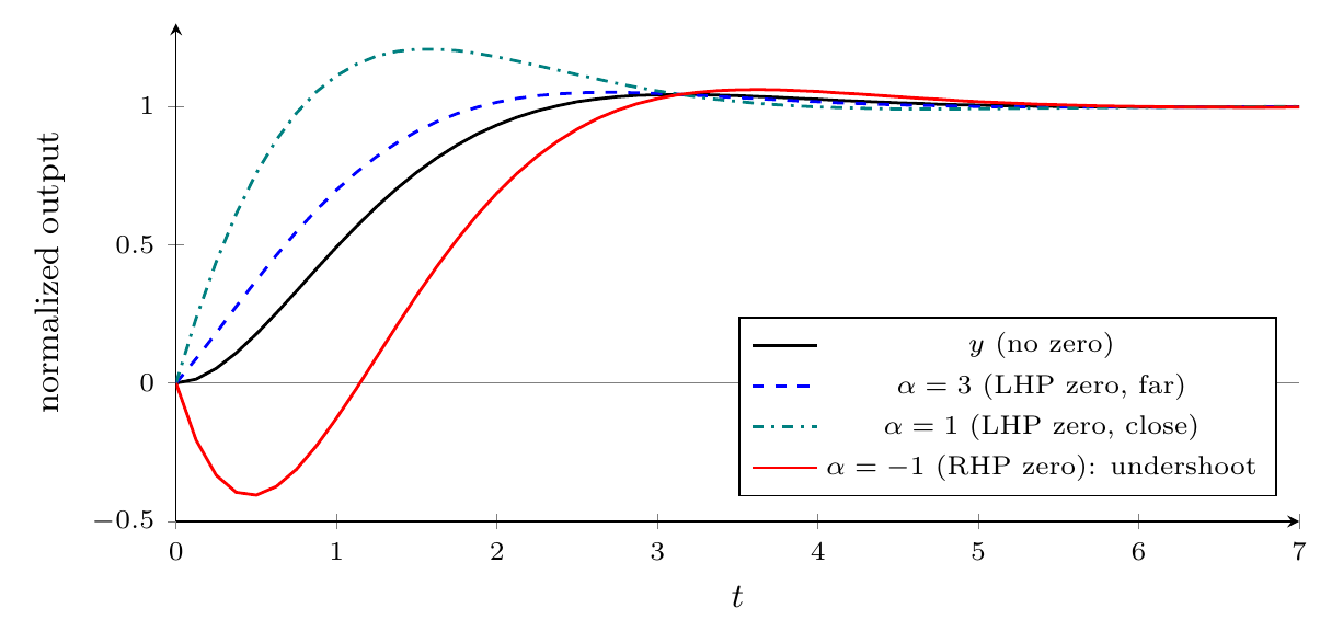
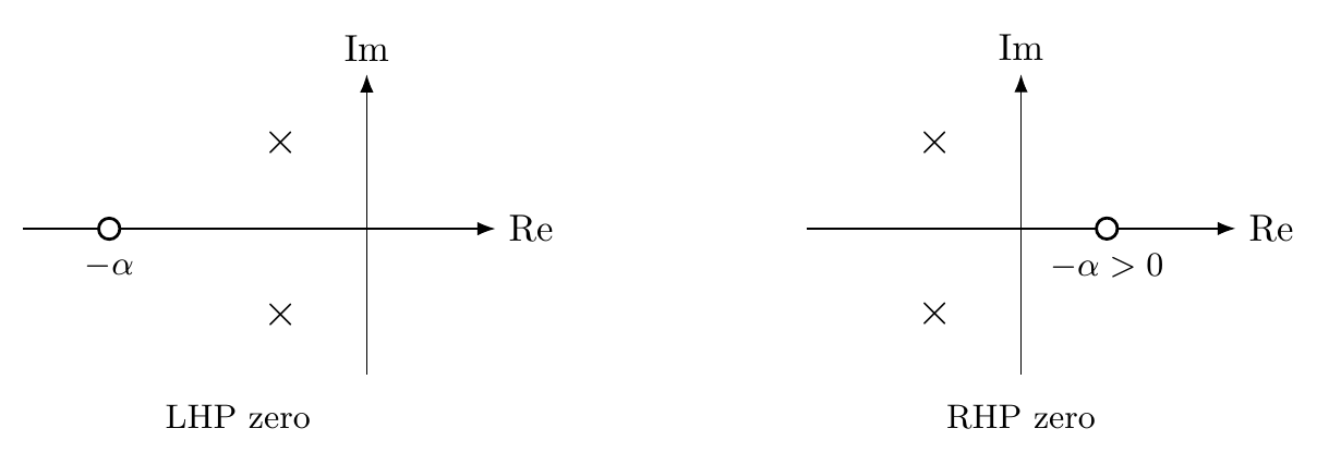
The four curves separate into two cases, according to where the zero sits:
A stable zero speeds up the rise
When $\alpha \gt 0$, the zero lies in the left half-plane. The scaled term $\alpha y$ keeps the original shape, and the derivative term, positive at the start, makes the output rise faster. After the first peak, the negative derivative reshapes the oscillation. How much the zero matters depends on its distance. A zero far to the left (large $\alpha$) makes $\dot y/\alpha$ small and changes little; a zero closer to the poles speeds up the rise more and adds overshoot. Lecture 17 uses exactly this effect to design faster controllers.
An unstable zero causes undershoot
When $\alpha \lt 0$, the zero lies in the right half-plane. Now $\alpha y$ is a mirror image of $y$; with $\alpha = -1$, for instance, it is $-y$. The derivative term is still positive at the start. Early on the derivative dominates, so the output moves away from its final value before it turns around. We distinguish two terms:
- Overshoot: going beyond the steady-state value.
- Undershoot: initially moving in the opposite direction to the steady-state value.
The steady state itself is unaffected, but the early transient changes completely.
The practical consequence is easy to picture. Command a motor to rotate to $+10^\circ$; if the transfer function has a right-half-plane zero, the motor first rotates the other way and only then turns back toward $+10^\circ$. Such systems are called non-minimum-phase, and they fundamentally limit how fast a controller can make the loop respond.
Summary and outlook
- A zero at $-\alpha$ gives $\tilde y = \alpha y + \dot y$: a scaled response plus a derivative term.
- A left-half-plane zero speeds up the rise, and more so the closer it is to the dominant poles.
- A right-half-plane zero causes undershoot: the response starts in the wrong direction.
We have now analyzed how poles and zeros shape the transient response, assuming the response settles at all. The next lecture makes that assumption precise: it defines stability and gives a test for it, the Routh-Hurwitz criterion, that needs no root computation.
References
- N. S. Nise, Control Systems Engineering, 6th ed.: §4.8 System Response With Zeros (p. 191).
- X. Chen and M. Tomizuka, Introduction to Modern Controls, with Illustrations in MATLAB and Python: §3.3 From Laplace Transform to Transfer Functions (p. 41).