Lecture 7: From Step Response to System Parameters
Lecture 6 introduced second-order systems and sorted their responses into four cases by the damping ratio. The underdamped case deserves a closer look: many physical systems are second order, many well-tuned feedback loops are underdamped, and, as later lectures show, many higher-order systems behave approximately like a second-order one. In this lecture we derive the exact step response of an underdamped second-order system ($0\lt \zeta\lt 1$), read off its key features, and then reverse the reasoning to identify a system’s parameters from a measured step response.
The spring–mass–damper
The standard example is a mass $m$ attached to a spring $k$ and a damper $b$, driven by a force $f$. Newton’s law gives
$$m\ddot x + b\dot x + kx = f \quad\Longrightarrow\quad G(s) = \frac{X(s)}{F(s)} = \frac{K\,\omega_n^2}{s^2 + 2\zeta\omega_n s + \omega_n^2}.$$Comparing coefficients with the standard form links the abstract parameters to the physical ones:
$$\omega_n = \sqrt{k/m},\qquad \zeta = \frac{b}{2\sqrt{km}},\qquad K = \frac{1}{k}.$$Here $\omega_n$ is the natural frequency, $\zeta$ the damping ratio and $K$ the static gain. We will also use the damped natural frequency $\omega_d = \omega_n\sqrt{1-\zeta^2}$.
The exact step response
Our goal is an explicit expression for $x(t)$ when $f$ is a unit step, $F(s)=1/s$. The approach is partial fractions, with the second-order factor written so that the Laplace-transform tables for cosine and sine apply directly. Completing the square in the denominator gives
$$X(s) = \frac{K\omega_n^2}{s\left[(s+\zeta\omega_n)^2 + \omega_d^2\right]} = K\left[\frac{k_1}{s} + \frac{k_2\,(s+\zeta\omega_n) + k_3\,\omega_d}{(s+\zeta\omega_n)^2+\omega_d^2}\right].$$The numerator of the second term is split into a part proportional to $(s+\zeta\omega_n)$, which will become a damped cosine, and a part proportional to $\omega_d$, which will become a damped sine.
The coefficient $k_1$ is the easy one. Multiplying both sides by $s$ and letting $s\to0$ (the cover-up method) gives $k_1 = \omega_n^2/\omega_n^2 = 1$. For $k_2$ and $k_3$ we put everything over the common denominator and match coefficients:
$$\omega_n^2 = (s^2 + 2\zeta\omega_n s + \omega_n^2) + k_2\,s(s+\zeta\omega_n) + k_3\,\omega_d\,s.$$The $s^2$ terms require $1 + k_2 = 0$, so $k_2=-1$. The $s^1$ terms require $2\zeta\omega_n + k_2\zeta\omega_n + k_3\omega_d = 0$, so $k_3 = -\zeta\omega_n/\omega_d$. The constant terms match automatically.
Taking the inverse Laplace transform, and using $\omega_n/\omega_d = 1/\sqrt{1-\zeta^2}$, we obtain
$$x(t) = K\left[1 - e^{-\zeta\omega_n t}\left(\cos\omega_d t + \frac{\zeta}{\sqrt{1-\zeta^2}}\sin\omega_d t\right)\right].\qquad(\star)$$Sine and cosine at the same frequency can be combined into one phase-shifted cosine, which gives a more compact form:
$$x(t) = K\left[1 - \frac{1}{\sqrt{1-\zeta^2}}\,e^{-\zeta\omega_n t}\cos(\omega_d t - \phi)\right], \qquad \phi = \arctan\frac{\zeta}{\sqrt{1-\zeta^2}}.$$This formula tells a clear story. The response consists of a step, which settles at the steady-state value $K$; an exponential envelope, which decays at a rate set by $\zeta\omega_n$; and an oscillation at the frequency $\omega_d$ inside that envelope.
Reading the response
With the exact formula in hand, we can read off the quantities engineers use to describe a step response:
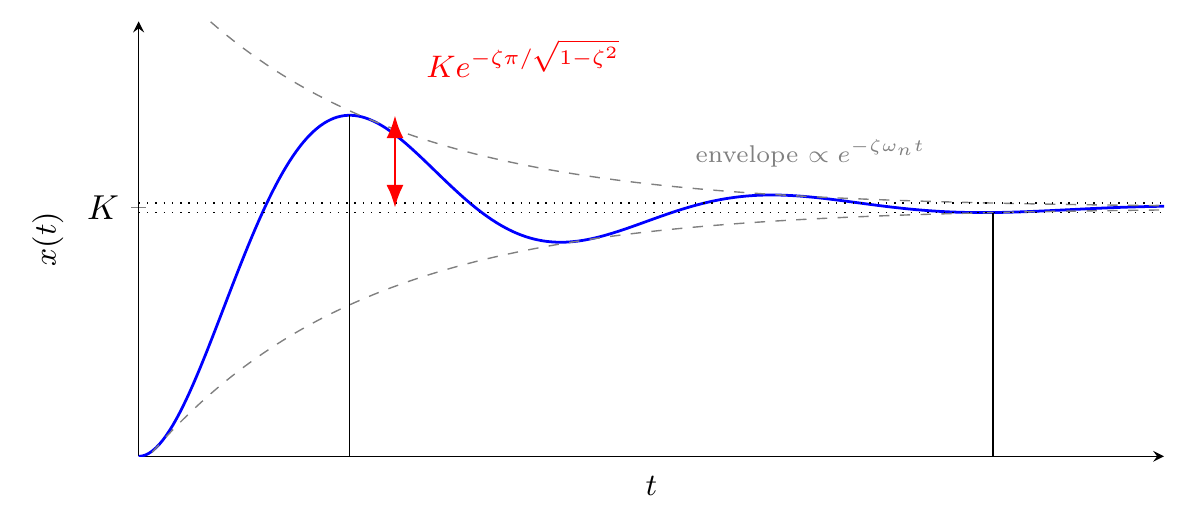
(Plotted for $\zeta = 0.3$, $\omega_n = 1$.)
The steady-state value is $K$. The envelope has time constant $\tau = 1/(\zeta\omega_n)$. After about four time constants the response stays within $\pm2\%$ of its final value, so the settling time is $T_s \approx 4/(\zeta\omega_n)$.
The oscillation has period $2\pi/\omega_d$, and the first peak comes after half a period, so the peak time is $T_p = \pi/\omega_d$. Substituting $t = \pi/\omega_d$ into ($\star$) is particularly easy, because $\cos\pi = -1$ and $\sin\pi = 0$:
$$x_{\max} = K\left(1 + e^{-\zeta\pi/\sqrt{1-\zeta^2}}\right).$$The response therefore exceeds its final value by $Ke^{-\zeta\pi/\sqrt{1-\zeta^2}}$. Dividing by the final value gives the percentage overshoot:
$$\%OS = e^{-\zeta\pi/\sqrt{1-\zeta^2}}\times 100\%.$$This depends only on the damping ratio, a fact that the root-locus design lectures rely on heavily.
Identifying a system from a step test
As engineers, we read these formulas in both directions. Suppose someone hands us the measured step response of a second-order system whose parameters are unknown. Its features are enough to identify it:
- Damping ratio from overshoot. Measure $\%OS$ from the graph. Taking logarithms, $\ln OS = -\zeta\pi/\sqrt{1-\zeta^2}$, and solving for $\zeta$ gives $$\zeta = \frac{-\ln(\%OS/100)}{\sqrt{\pi^2 + \ln^2(\%OS/100)}}.$$
- Natural frequency from peak time. Measure $T_p$, so $\omega_d = \pi/T_p$. Then $\omega_n = \omega_d/\sqrt{1-\zeta^2}$.
- Physical parameters. With $K = 1/k$, $\omega_n = \sqrt{k/m}$ and $\zeta = b/(2\sqrt{km})$, we can recover $k$, $m$ and $b$.
For example, an overshoot of $20\%$ gives $\zeta = 1.609/\sqrt{9.870 + 2.590} = 0.456$. This value reappears in Lecture 19.
Summary and outlook
- Partial fractions give the exact step response: cover-up for $k_1$, matching coefficients for $k_2$ and $k_3$.
- $\zeta\omega_n$ sets the decay (settling time), $\omega_d$ sets the oscillation (peak time), and $\zeta$ alone sets the overshoot.
- The same formulas, read in reverse, identify $\zeta$ and $\omega_n$ from a single step test.
Real systems are rarely exactly second order. The next lecture shows when a higher-order system still behaves like a second-order one, through the idea of dominant poles.
References
- N. S. Nise, Control Systems Engineering, 6th ed.: §4.4 Second-Order Systems: Introduction (p. 168); §4.5 The General Second-Order System (p. 173); §4.6 Underdamped Second-Order Systems (p. 177).
- X. Chen and M. Tomizuka, Introduction to Modern Controls, with Illustrations in MATLAB and Python: §3.2 Inverse Laplace Transform and Partial Fraction Expansion (p. 39).