Lecture 25: Nyquist Plots with Imaginary-Axis Poles: Contour Detours

Scheduled release: week of November 16, 2026.

Download lecture notes (PDF)

Introduction

The ordinary Nyquist contour follows the imaginary axis and closes through the right half-plane. This construction needs modification when an open-loop pole lies on the imaginary axis, because a contour used in the argument principle cannot pass through a pole. Small detours keep the mapping finite before a limit is taken. The examples below show how to map those detours for an integrator, a double integrator, and poles at nonzero imaginary frequencies. The stability convention remains $Z=P-N_{\mathrm{CCW}}$, where $P$ counts poles strictly inside the modified contour.

A pole approaching the origin

A useful way to approach an imaginary-axis pole is to move a stable real pole toward the origin. For $L(s)=1/(s+a)$ with $a\gt 0$, the ordinary Nyquist image is a circle. Following this family as $a$ decreases reveals which part of the image becomes singular in the integrator limit.

$$ L(j\omega)=\frac{a-j\omega}{a^2+\omega^2},\qquad \left(\Re L-\frac{1}{2a}\right)^2+(\Im L)^2=\frac{1}{4a^2}. $$

Compare $a=10,1,0.5$ before considering the integrator. The circle expands as $a$ decreases. At any fixed nonzero frequency, the limit is $1/(j\omega)$. This limit is not uniform near zero frequency: part of the circle moves to infinity. An integrator is not BIBO stable; the phrase marginal pole refers here to its location on the imaginary axis.

Why the origin needs a detour

The expanding circle shows why simply setting $a=0$ loses information near zero frequency. The finite-frequency limit exists away from the origin, but a portion of the image moves without bound. We need a contour that avoids the singular point while preserving the connection between the branches.

$$ \begin{aligned}a\gt 0:&\quad L(0)=1/a,\\a\to0^+:&\quad 1/a\to\infty,\\a=0:&\quad L(j\omega)=-j/\omega.\end{aligned} $$

The examples $a=10,1,0.5$ start at $0.1,1,2$ on the real axis. Their Nyquist circles grow as the pole moves toward the origin. In the integrator limit, the finite-frequency branches approach the imaginary axis, but a connection remains at infinity. Simply substituting $\omega=0$ is impossible. A small detour makes every point of the contour finite first, so that its image and orientation can be determined before taking a limit.

Indent the contour around a boundary pole

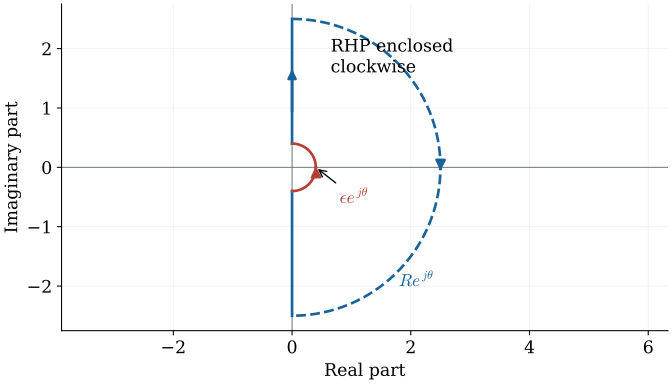
A small semicircular indentation into the right half-plane supplies that connection in the domain. It excludes the boundary pole from the enclosed region and avoids evaluating the transfer function at the pole itself. The detour must be mapped before its radius is allowed to tend to zero.

$$ L(s)=\frac{L_0(s)}{s},\qquad s=\epsilon e^{j\theta},\qquad -\frac{\pi}{2}\leq\theta\leq\frac{\pi}{2}. $$

Traverse the indentation from $-j\epsilon$ to $+j\epsilon$, counterclockwise around the excluded pole. The rest of the overall right-half-plane contour retains its clockwise orientation. Count strictly right-half-plane poles inside the modified contour; the excluded boundary pole is not added to $P$. Take $R\to\infty$ and $\epsilon\to0^+$ only after the complete mapped contour has been constructed.

The straight branches of an integrator

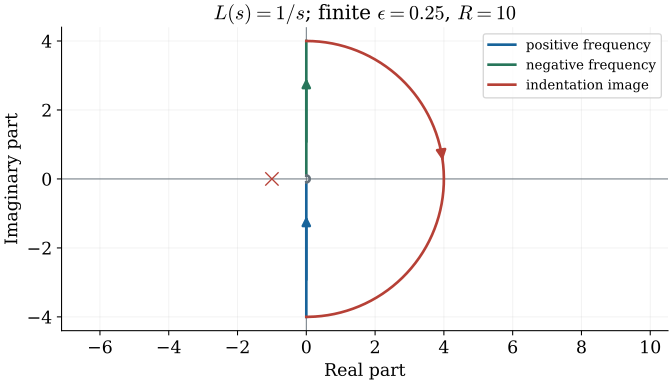
With the modified contour specified, begin by mapping its straight imaginary-axis segments for the integrator $L(s)=1/s$. These give the familiar frequency branches. They must then be connected by the images of the large outer semicircle and the small indentation.

$$ L(j\omega)=-\frac{j}{\omega},\qquad L(Re^{j\theta})=\frac{1}{R}e^{-j\theta}\longrightarrow0. $$

The positive-frequency branch moves from a large negative imaginary value toward zero. The negative-frequency branch is the conjugate reflection, traversed from near zero toward a large positive imaginary value. The large domain semicircle maps to a small arc near the origin. The missing connection is supplied by the indentation, not by an arbitrary line.

A small domain arc maps to a large image arc

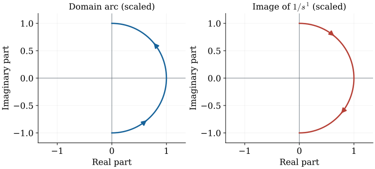
The missing distant connection comes from the indentation. Near a simple pole at the origin, write $L(s)=L_0(s)/s$ with $L_0(0)\ne0$. Substituting the small semicircle shows that its radius is inverted and its angular direction is reversed.

$$ L(\epsilon e^{j\theta})\sim\frac{L_0(0)}{\epsilon}e^{-j\theta}. $$

For the integrator, $L_0(0)=1$. The image angle decreases from $+90^\circ$ to $-90^\circ$, yielding a clockwise right semicircle of radius $1/\epsilon$. If $L_0(0)$ is another nonzero number, its magnitude scales the arc and its phase rotates it. With unity negative feedback, $1/s$ gives $T=1/(s+1)$, a stable closed-loop check of the full contour.

Track the four segment endpoints

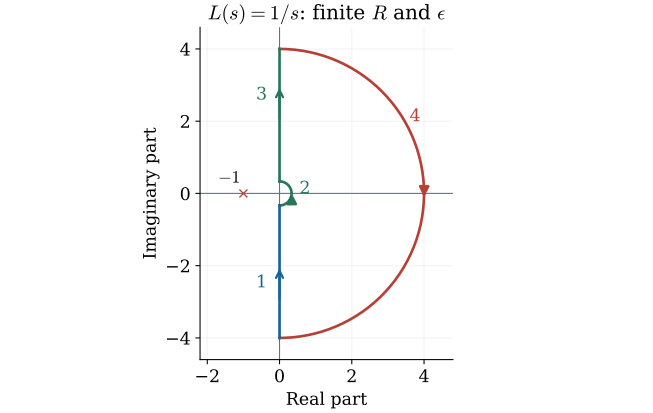
The full integrator image is now determined, but tracking the segment endpoints makes its orientation easier to verify. Both domain semicircles map to image semicircles, with radii inverted. The two arcs connect the positive- and negative-frequency branches at different scales.

$$ \begin{aligned}\Gamma_1:&\ -j/\epsilon\ \to -j/R,\\\Gamma_2:&\ -j/R\ \to +j/R,\\\Gamma_3:&\ +j/R\ \to +j/\epsilon,\\\Gamma_4:&\ +j/\epsilon\ \to -j/\epsilon.\end{aligned} $$

For $L=1/s$, the two imaginary-axis pieces are joined by two right semicircles: a small one of radius $1/R$ and a large one of radius $1/\epsilon$. On $\Gamma_2$, the domain angle decreases, so the image angle increases from $-\pi/2$ to $+\pi/2$. On $\Gamma_4$, the domain angle increases, so the image angle decreases from $+\pi/2$ to $-\pi/2$. Keeping both arcs resolves the apparent missing connection.

A repeated stable pole

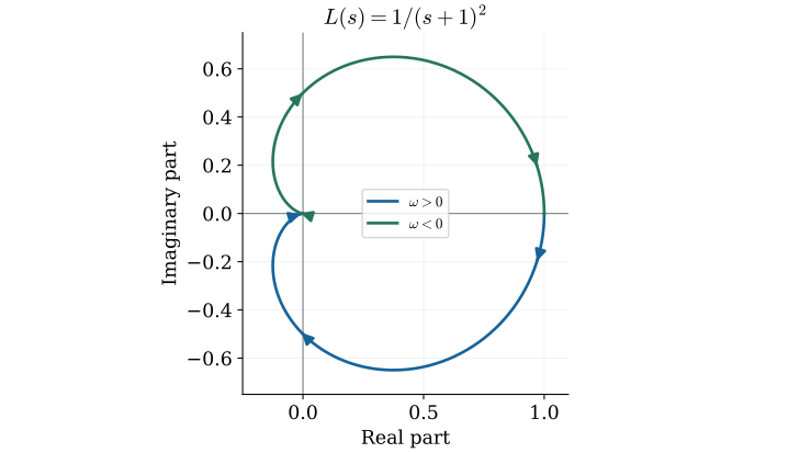
Before increasing the boundary-pole multiplicity, consider a repeated pole that remains in the left half-plane. The loop $1/(s+1)^2$ needs no indentation, but its two denominator factors double the high-frequency phase contribution. This separates the effect of multiplicity from the need to modify the contour.

$$ L(j\omega)=\frac{1-\omega^2-2j\omega}{(1+\omega^2)^2},\qquad \angle L(j\omega)=-2\tan^{-1}\omega. $$

The curve starts at $1$ and approaches the origin from below along the negative-real direction: its phase tends to $-180^\circ$, not $-90^\circ$. Under unity feedback the characteristic roots are $-1\pm j$, confirming stability.

A double pole at the origin

Moving both poles to the origin introduces both effects at once. For $L(s)=1/s^2$, the frequency branches lie on the negative real axis, while the indentation image makes a full turn. The complete traversal is therefore essential even though the finite-frequency sketch looks simple.

$$ L(j\omega)=-\frac{1}{\omega^2},\qquad L(\epsilon e^{j\theta})=\epsilon^{-2}e^{-2j\theta}. $$

Both frequency branches lie on the negative real axis, with opposite traversal directions. Across the indentation, $\theta$ increases by $\pi$ and the image phase decreases by $2\pi$: a full clockwise turn at large radius. More generally, $L_0(s)/s^m$ contributes an image phase change of $-m\pi$ on that detour if $L_0(0)\ne0$. For unity feedback, $1/s^2$ has characteristic roots $\pm j$; the frequency curve passes through $-1$ at $\omega=1$, so strict asymptotic stability is not obtained.

Double integrator: twice the angular change

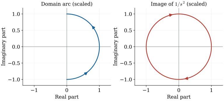
The full turn can be verified directly from the angular parameter. A semicircle changes the domain angle by $\pi$; the reciprocal-square factor changes the image angle by $-2\pi$. The starting and ending image points coincide geometrically, but the unwrapped angle records the intervening rotation.

$$ \begin{aligned}s&=\epsilon e^{j\theta},\quad\theta:-\pi/2\to\pi/2,\\s^{-2}&=\epsilon^{-2}e^{-2j\theta},\\\arg(s^{-2})&:\quad \pi\to-\pi.\end{aligned} $$

The negative-frequency straight segment ends at $-1/\epsilon^2$, on the negative real axis. The indentation starts there with unwrapped angle $\pi$ and finishes at the same geometric point with angle $-\pi$. Thus it contributes a full clockwise turn, not a half circle. The two straight branches overlap geometrically but run in opposite directions. Their coincident appearance must not erase either part of the traversal.

Poles away from the origin on the imaginary axis

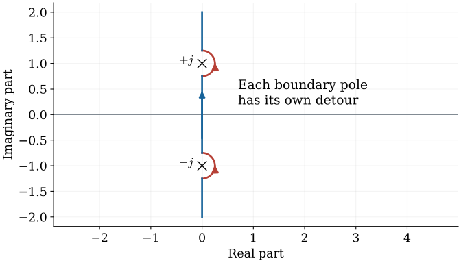
The same local reasoning applies to a boundary pole away from the origin. For $L(s)=1/(s^2+1)$, separate detours are required around $+j$ and $-j$. Expanding about each pole gives a reciprocal local coordinate, multiplied by a coefficient that rotates and scales the image arc.

$$ s=-j+\epsilon e^{j\theta},\qquad s^2+1=-2j\epsilon e^{j\theta}+\epsilon^2e^{2j\theta}. $$

The term linear in $\epsilon$ dominates the quadratic term as the detour shrinks. Therefore $L(s)\sim[-2j\epsilon e^{j\theta}]^{-1}$. A matching detour is needed around $+j$. Track the local residue as well as the inverse radius; it determines the orientation and phase offset of each large image arc. Under unity feedback, the characteristic equation is $s^2+2=0$, with imaginary-axis roots $\pm j\sqrt{2}$. This is a boundary case, not asymptotic stability.

Expand locally about the pole at minus j

To see that coefficient explicitly, expand first about $s=-j$. The constant denominator terms cancel at the pole, leaving a leading term proportional to the detour radius. The corresponding calculation about $+j$ gives the companion arc with its own phase offset.

$$ \begin{aligned}s&=-j+\epsilon e^{j\theta},\\s^2+1&=(-j)^2-2j\epsilon e^{j\theta}\\&\hspace{8mm}+\epsilon^2e^{2j\theta}+1,\\L(s)&\sim\frac{j}{2\epsilon}e^{-j\theta}.\end{aligned} $$

The constant terms $(-j)^2$ and $1$ cancel. The term of order $\epsilon$ dominates the term of order $\epsilon^2$, leaving the local coefficient $j/2$. The image has radius approximately $1/(2\epsilon)$ and angle $\pi/2-\theta$. Around $+j$, the coefficient is $-j/2$, so the companion arc has angle $-\pi/2-\theta$. Each detour reverses its angular direction in the image, with a different phase offset.

Perspective

The detours preserve a valid contour while retaining the information that would otherwise disappear at a singular frequency. Their mapped arcs are determined by the local pole order and coefficient, so they must be included in the complete winding calculation. After the contour is assembled, apply the usual root count and check separately for closed-loop roots on the imaginary axis.

The next lecture uses axis crossings to construct a higher-order Nyquist curve and determine how changing the loop gain affects stability.

References

Norman S. Nise, Control Systems Engineering, 6th ed., Wiley, 2011.

• §§10.4–10.5: Nyquist diagrams, contour detours, and stability.