Lecture 20: Bode Plots: Sinusoidal Response, Magnitude and Phase

Download lecture notes (PDF)

Introduction

A frequency response describes how a linear time-invariant (LTI) system changes the amplitude and phase of a sinusoidal input. This description provides a useful bridge between a transfer function and the response to commands, disturbances, and noise. We first derive the sinusoidal response of a stable system, then use complex-number geometry to obtain the same result directly. Factoring the transfer function leads to the elementary pole and zero curves from which Bode plots are constructed. Unless stated otherwise, the response calculations assume zero initial conditions.

Why decompose an input into frequencies?

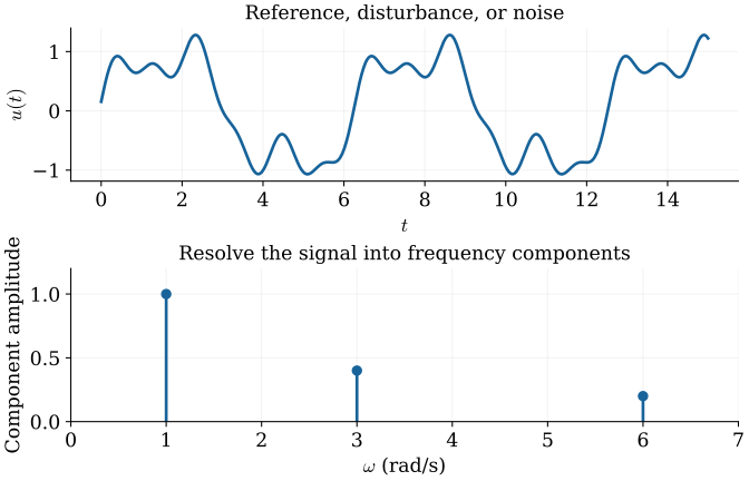
A complicated input is easier to analyze when it is expressed in terms of simpler components. For signals that admit a sinusoidal expansion, linearity allows us to study each component separately and add the resulting outputs. The following representation makes the amplitude, frequency, and phase of each component explicit.

$$ u(t)=\sum_i M_i\sin(\omega_i t+\phi_i). $$

Overshoot and settling time describe responses to standard test signals such as a step. In practice, a command may have a more complicated shape, and disturbances or noise may contain many frequencies. A time trace alone may hide where its frequency content is concentrated. For an LTI system, superposition lets us analyze one sinusoidal component and then combine the responses. The input may be chosen by a designer or imposed by the environment. Angular frequency is measured in rad/s, with $\omega=2\pi f$ when $f$ is in hertz.

A single sinusoid in the Laplace domain

It is therefore enough to begin with one sinusoid. Let $M_i$, $\omega_i$, and $\phi_i$ denote its amplitude, angular frequency, and phase. The Laplace transform reveals how the poles introduced by this forcing interact with the poles of the system.

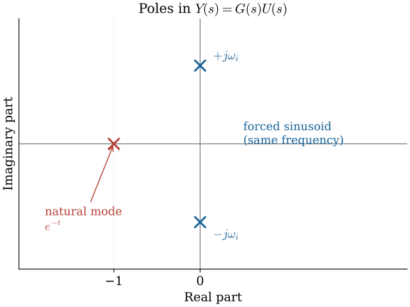
$$ \begin{aligned}u(t)&=M_i\sin(\omega_i t+\phi_i),\quad t\ge0,\\U(s)&=M_i\frac{s\sin\phi_i+\omega_i\cos\phi_i}{s^2+\omega_i^2},\\Y(s)&=G(s)U(s).\end{aligned} $$

Expand the shifted sine into a sine and a cosine. Both Laplace transforms contain the same denominator $s^2+\omega_i^2$, giving poles at $\pm j\omega_i$. Multiplication by $G(s)$ adds the system poles. Partial fractions therefore separate a term at the input frequency from terms associated with the natural modes. This separation explains why the steady-state output keeps the input frequency.

Separate transient and steady-state responses

The two sets of poles have different meanings in the time domain. System poles generate natural modes, whereas the input poles generate the forced sinusoid. If the system is asymptotically stable, the natural modes decay and leave the steady-state response.

$$ y(t)=M_o\sin(\omega_i t+\phi_o)+y_{\mathrm{tr}}(t),\qquad y_{\mathrm{tr}}(t)\to0. $$

This steady-state interpretation assumes stable poles and no singularity at the forcing frequency. Partial fractions separate terms due to the system poles from terms at the input frequencies $\pm j\omega_i$. Stable real modes decay exponentially, and stable complex modes decay while oscillating. An unstable system need not settle to a bounded sinusoid, even though its algebraic frequency response may still be evaluated.

First-order partial fractions

A first-order example makes this separation explicit. Choose $G(s)=1/(s+1)$ and a unit sinusoid of angular frequency $\omega$. Partial fractions isolate the natural mode at $s=-1$ from the forced modes at $s=\pm j\omega$.

$$ \begin{aligned}G(s)&=\frac{1}{s+1},\quad U(s)=\frac{\omega}{s^2+\omega^2},\\Y(s)&=\frac{\omega}{1+\omega^2}\frac1{s+1}\\&\quad+\frac{-\omega s+\omega}{(1+\omega^2)(s^2+\omega^2)}.\end{aligned} $$

Take a unit sine input with zero phase. Write $Y=A/(s+1)+(Bs+C)/(s^2+\omega^2)$ and multiply through by the common denominator. Equating powers of $s$ gives $A+B=0$, $B+C=0$, and $A\omega^2+C=\omega$. Thus $A=C=\omega/(1+\omega^2)$ and $B=-\omega/(1+\omega^2)$. The first term is the decaying system mode; the second contains sine and cosine at the forcing frequency.

The transient decays; the sinusoid remains

The partial-fraction expression can now be transformed back to time. Its exponential term is the transient; the remaining sine and cosine can be combined into one sinusoid. This combination gives the output amplitude and phase lag directly.

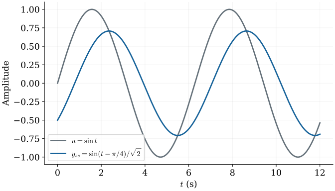
$$ \begin{aligned}y(t)&=\frac{\omega e^{-t}+\sin\omega t-\omega\cos\omega t}{1+\omega^2},\\y_{\mathrm{ss}}(t)&=\frac{\sin(\omega t-\tan^{-1}\omega)}{\sqrt{1+\omega^2}}.\end{aligned} $$

The first term tends to zero because the system pole is at $-1$. Combine the remaining sine and cosine into one sine with a phase lag: if $\alpha=\tan^{-1}\omega$, then $\cos\alpha=1/\sqrt{1+\omega^2}$ and $\sin\alpha=\omega/\sqrt{1+\omega^2}$. This gives the amplitude ratio and phase directly. At $\omega=1$, the response has amplitude $1/\sqrt2$ and lag $\pi/4$.

Magnitude scales amplitude; phase shifts timing

The first-order calculation suggests a much shorter description of sinusoidal steady state. For any asymptotically stable LTI system, evaluating the transfer function at the forcing frequency gives the amplitude ratio and phase shift, provided the evaluation is finite. Thus the input and output are related by the following two quantities.

$$ M_o=M_i|G(j\omega_i)|,\qquad \phi_o=\phi_i+\arg G(j\omega_i). $$

For the example $G(s)=1/(s+1)$, the gain is $1/\sqrt{1+\omega_i^2}$ and the phase is $-\tan^{-1}\omega_i$. At $\omega_i=1$ rad/s, a unit-amplitude sinusoid becomes a sinusoid of amplitude $1/\sqrt{2}$ with a $45^\circ$ lag.

Read gain and phase from a complex vector

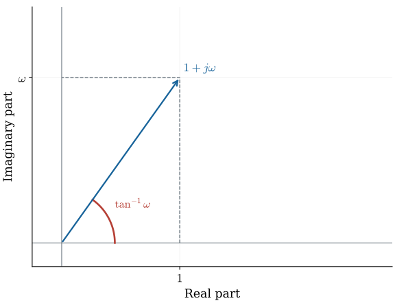
To see why this description is efficient, return to $G(s)=1/(s+1)$. The denominator at $s=j\omega_i$ is a vector in the complex plane. Taking its reciprocal produces the gain and phase already obtained through partial fractions.

$$ \begin{aligned}G(j\omega_i)&=\frac1{1+j\omega_i},\\|G(j\omega_i)|&=\frac1{\sqrt{1+\omega_i^2}},\\\arg G(j\omega_i)&=-\tan^{-1}\omega_i.\end{aligned} $$

The denominator vector has horizontal component one and vertical component $\omega_i$. Its length is $\sqrt{1+\omega_i^2}$ and its angle is $\tan^{-1}\omega_i$. Division takes the reciprocal of that length and subtracts that angle from the numerator angle, which is zero. This repeats the partial-fraction result with much less computation and extends immediately to any input amplitude and initial phase.

Factor a general transfer function

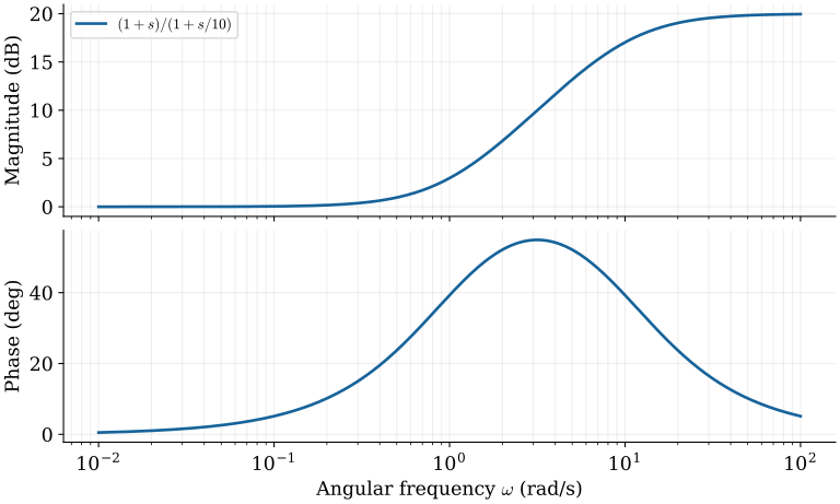
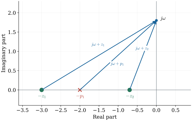
The same vector calculation extends to a transfer function with several poles and zeros. Factor the numerator and denominator so that each root contributes one elementary vector. The full response can then be assembled from the magnitudes and angles of these factors.

$$ G(s)=K\frac{\prod_i(s+z_i)}{\prod_k(s+p_k)},\qquad \arg G=\arg K+\sum_i\arg(j\omega+z_i)-\sum_k\arg(j\omega+p_k). $$

The magnitude is the product of numerator magnitudes divided by the product of denominator magnitudes. A positive constant gain contributes zero phase; a negative gain contributes $180^\circ$ modulo $360^\circ$. Use a quadrant-aware argument for general complex factors. The following real-pole and real-zero formulas assume positive $z_i$ and $p_k$; nonminimum-phase factors require their own phase treatment.

Magnitude and phase of a product

The reason this factor-by-factor construction works is most transparent in polar form. Each complex number has a magnitude and an angle, so products multiply magnitudes and add angles. Denominator factors enter through division and therefore subtract their angles.

$$ \begin{aligned}G(j\omega)&=K\frac{\prod_i(j\omega+z_i)}{\prod_k(j\omega+p_k)},\\|G|&=|K|\frac{\prod_i|j\omega+z_i|}{\prod_k|j\omega+p_k|},\\\arg G&=\arg K+\sum_i\phi_{z_i}-\sum_k\phi_{p_k}.\end{aligned} $$

A complex factor is its magnitude multiplied by an exponential of its angle. Multiplying such exponentials adds angles, while division subtracts angles. The scalar $K$ contributes magnitude $|K|$; its phase is zero for positive gain and $180^\circ$ for negative gain. This reduction is why first-order factors are useful building blocks: once their curves are known, the full response can be assembled graphically.

A real zero: low, corner, and high frequency

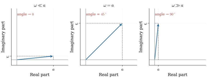
We can now develop the simplest nonconstant building block: a real zero at $s=-a$, with $a\gt 0$. Evaluating $s+a$ along the imaginary axis gives a vector with a fixed horizontal component and a frequency-dependent vertical component. Its limiting geometry determines the shape of the response.

$$ |a+j\omega|=\sqrt{a^2+\omega^2},\qquad \phi=\tan^{-1}(\omega/a). $$

For $\omega\ll a$, the magnitude is approximately $a$ and the phase approximately zero. For $\omega\gg a$, the magnitude is approximately $\omega$ and the phase approaches $90^\circ$. At $\omega=a$, the magnitude is $a\sqrt{2}$ and the phase is $45^\circ$. A straight-line phase approximation ramps over $0.1a$ to $10a$. The exact endpoint angles are about $5.71^\circ$ and $84.29^\circ$, so the flat ends are approximations. Figures use $a=1$.

Construct the zero from three frequency regions

Rather than calculating many points, we can anchor the zero’s response in three frequency regions. The low-frequency and high-frequency limits identify the asymptotes, while the corner $\omega=a$ connects them. These checks also show why the ratio $\omega/a$ controls the transition.

$$ \begin{array}{c|c|c}\omega&|a+j\omega|&\arg(a+j\omega)\\\hline\omega\ll a&a&0\\\omega=a&a\sqrt2&45^\circ\\\omega\gg a&\omega&90^\circ\end{array} $$

At low frequency the horizontal component $a$ dominates. At high frequency the vertical component $\omega$ dominates. At the corner, the two components are equal, so the vector makes a $45^\circ$ angle and has length $a\sqrt2$. These three checks locate the smooth magnitude and phase curves. The ratio $\omega/a$, rather than the absolute size of either quantity, controls the transition.

The two-decade phase approximation

The exact phase curve is smooth, but a straight-line approximation is convenient for hand sketches. We construct it from the two frequency decades surrounding the corner. This phase interval is wider than the single breakpoint used for the magnitude asymptotes.

$$ \phi_z(\omega)\approx\begin{cases}0,&\omega\le0.1a,\\45^\circ[1+\log_{10}(\omega/a)],&0.1a\lt \omega\lt 10a,\\90^\circ,&\omega\ge10a.\end{cases} $$

The exact phase at $0.1a$ is about $5.71^\circ$, and at $10a$ it is about $84.29^\circ$. Approximating these endpoints by zero and $90^\circ$ produces a straight ramp across two decades. The ramp passes exactly through $45^\circ$ at $a$. The magnitude asymptotes instead intersect at the single corner $a$. Do not confuse the phase transition interval with the magnitude breakpoint.

A real pole is the reciprocal building block

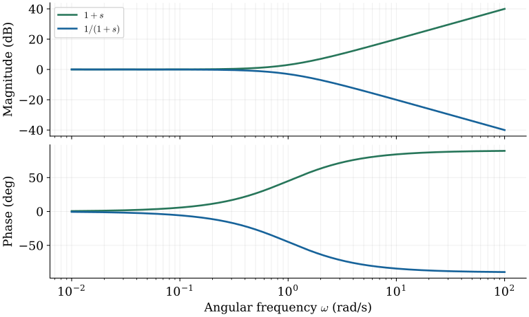
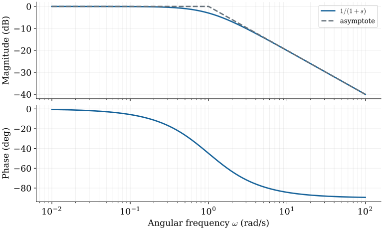
Once the zero factor is understood, a stable real pole follows by taking its reciprocal. The reciprocal reduces the magnitude and reverses the phase angle. Care is needed with the constant factor, because $1/(s+a)$ and $1/(1+s/a)$ have different DC gains.

$$ \left|\frac{1}{a+j\omega}\right|=\frac{1}{\sqrt{a^2+\omega^2}},\qquad \phi=-\tan^{-1}(\omega/a). $$

The low-frequency magnitude is $1/a$. The high-frequency magnitude is $1/\omega$. At the corner it is $1/(a\sqrt{2})$, and the phase is $-45^\circ$. For the normalized pole $1/(1+s/a)$, the DC gain is one and the exact corner magnitude is $-3.0103$ dB. Keep this normalization distinct from the unnormalized factor $1/(s+a)$.

Why Bode plots use logarithms

Products of many factors are cumbersome on a linear magnitude scale. Taking a logarithm converts those products into sums, while a logarithmic frequency axis accommodates a wide range of time scales. This gives the conventional Bode magnitude representation in decibels.

$$ M_{\mathrm{dB}}=20\log_{10}|G(j\omega)|,\qquad 20\log_{10}|G_1G_2|=20\log_{10}|G_1|+20\log_{10}|G_2|. $$

A decade is a tenfold frequency increase. A factor proportional to $\omega$ adds $20$ dB per decade; a factor proportional to $1/\omega$ adds $-20$ dB per decade. The horizontal axis is logarithmic in frequency, while the vertical magnitude axis is linear in the dB quantity. This makes the slope changes of a multi-factor system easy to combine. These rules extend to products of many factors.

A reciprocal becomes a reflection in decibels

The reciprocal relation between a zero and a pole becomes especially simple in decibels. Since the logarithm of a reciprocal changes sign, the two magnitude curves are reflections when their normalizations match. Their phase contributions likewise have opposite signs.

$$ \begin{aligned}20\log_{10}\frac1{|a+j\omega|}&=-20\log_{10}|a+j\omega|,\\\arg\frac1{a+j\omega}&=-\arg(a+j\omega),\\20\log_{10}(10\omega)-20\log_{10}\omega&=20\ {\mathrm{dB}}.\end{aligned} $$

Taking a reciprocal reflects the logarithmic magnitude about zero dB and the phase about zero degrees, provided the same normalization is used. A tenfold frequency increase is one decade. Where the zero magnitude is approximately proportional to frequency, each decade adds 20 dB; for a pole it subtracts 20 dB. Logarithmic frequency also allows a wide range of frequencies to fit on one axis.

Perspective

The sinusoidal calculation has reduced a time-domain response to the magnitude and angle of $G(j\omega)$. Factoring $G$ then reduces that complex calculation to elementary pole and zero contributions. On Bode axes, magnitude contributions add in decibels and phase contributions add as angles. These rules provide the starting point for combining several factors and understanding compensator behavior.

The next lecture combines these elementary factors and examines the effect of damping on a second-order frequency response.

References

Norman S. Nise, Control Systems Engineering, 6th ed., Wiley, 2011.

• §§10.1–10.2: Frequency response and Bode plots.