Lecture 21: Bode Plots: Phase Lead, Multiple Poles and Resonance

Scheduled release: week of November 16, 2026.

Download lecture notes (PDF)

Introduction

Bode plots become useful for design when the contributions of several poles and zeros can be combined without calculating every frequency point. A stable real zero contributes positive phase, whereas a stable real pole contributes negative phase; in decibels, their magnitude contributions add. We use these rules to explain lead and lag compensation and to assemble responses with several real factors. We then consider a complex pole pair, for which damping determines the shape of the response near resonance.

First-order building blocks

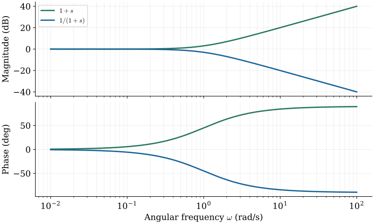
The construction starts with the real factors already encountered in sinusoidal-response analysis. A zero at $-a$ and a pole at $-a$ have the same corner frequency, but their effects on magnitude slope and phase have opposite signs. Keeping these two rules separate avoids confusing decibel slopes with angular slopes.

$$ G_z(s)=s+a,\qquad G_p(s)=\frac{1}{s+a},\qquad a\gt 0. $$

A zero changes the asymptotic magnitude slope by $+20$ dB/decade at $a$; a pole changes it by $-20$ dB/decade. The phase changes over approximately $0.1a$ to $10a$. Its ramp slope is $+45^\circ$/decade for the zero and $-45^\circ$/decade for the pole. Magnitude-slope units are dB/decade; phase-slope units are degrees/decade.

Why a lead compensator produces phase lead

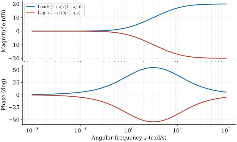
Combining one zero and one pole gives a simple compensator. If the zero has the lower break frequency, its positive phase contribution appears before the pole’s negative contribution. The resulting phase lead explains how the ordering of the roots affects the loop response.

$$ C(s)=K\frac{s+z}{s+p},\qquad 0\lt z\lt p,\qquad \phi_C=\tan^{-1}(\omega/z)-\tan^{-1}(\omega/p). $$

For positive $K$, the phase is positive between the low- and high-frequency limits. A lag compensator reverses the ordering, $0\lt p\lt z$, and contributes negative phase. Here $z,p$ are positive magnitudes of left-half-plane root locations. The curves show the ordering with break frequencies 1 and 10 rad/s.

Place the zero before the pole for phase lead

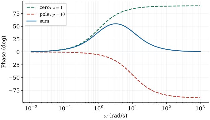
This ordering can be checked directly from the phase formula. For a positive frequency and $z\lt p$, the zero’s arctangent is larger than the pole’s arctangent. The difference is therefore positive, even though it tends to zero at both frequency extremes.

$$ \begin{aligned}\phi_z&=\tan^{-1}(\omega/z),\\\phi_p&=-\tan^{-1}(\omega/p),\\0\lt z\lt p&\ \Longrightarrow\ \phi_z+\phi_p\gt 0.\end{aligned} $$

With $z\lt p$, the ratio $\omega/z$ is larger than $\omega/p$ at every positive frequency. Since arctangent is increasing, the zero contribution exceeds the magnitude of the pole contribution. Both contributions vanish at low frequency and cancel as frequency tends to infinity, leaving a positive phase bump between them. Reversing their order gives a lag compensator. This frequency-domain picture explains the names lead and lag.

Add magnitude slopes at each breakpoint

The compensator example combines two factors of opposite type. The same addition rule applies to any collection of poles and zeros: order the break frequencies, establish the initial gain, and update the accumulated magnitude slope at each break.

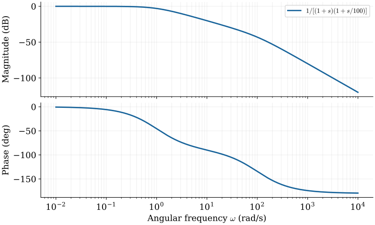
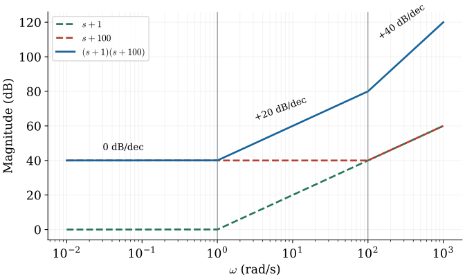
$$ 20\log_{10}|(j\omega+a_1)(j\omega+a_2)|=20\log_{10}|j\omega+a_1|+20\log_{10}|j\omega+a_2|. $$

With $a_1\lt a_2$, two zeros produce slopes $0$, $+20$, then $+40$ dB/decade. Two poles produce $0$, $-20$, then $-40$ dB/decade. Establish the correct low-frequency gain before tracing these slope changes. Normalizing each factor as $a(1+s/a)$ is a reliable way to keep the constant gain. The figure uses normalized poles at 1 and 100 rad/s.

Two zeros: add the individual lines

For a concrete construction, consider two real zeros with $a_1\lt a_2$. Below both break frequencies, each contributes an approximately constant magnitude. As the frequency passes each corner, one more rising asymptote contributes to the total.

$$ \begin{aligned}G_1(s)&=(s+a_1)(s+a_2),\quad a_1\lt a_2,\\M_1&=20\log_{10}|j\omega+a_1|,\\M_2&=20\log_{10}|j\omega+a_2|,\\M_{G_1}&=M_1+M_2.\end{aligned} $$

Below both corners, the magnitude is approximately $a_1a_2$, so the line begins at $20\log_{10}(a_1a_2)$. Crossing $a_1$ activates the first $+20$ dB/decade contribution. Crossing $a_2$ activates the second, giving $+40$ dB/decade. Add the two ordinates at each frequency, rather than joining unrelated line segments. The reciprocal two-pole model reflects the complete magnitude construction in zero dB.

Add phase ramps, including overlap

The magnitude construction is only half of the Bode plot. Phase must also be added at each frequency, but its transition intervals extend on both sides of the magnitude corners. Consequently, phase contributions can overlap even when the break frequencies are distinct.

$$ \phi(\omega)=-\tan^{-1}(\omega/a_1)-\tan^{-1}(\omega/a_2). $$

For two stable real poles, the total phase tends to $-180^\circ$. If their transition intervals overlap, the ramp slopes add in the overlap; they are not two isolated steps. Two zeros similarly approach $+180^\circ$.

Build phase from the transition intervals

To make that overlap explicit, mark the beginning and end of every phase ramp before adding the curves. A factor contributes a changing angle only within its own approximate transition interval. In an overlap, both ramp slopes contribute to the total.

$$ \begin{aligned}(M_1e^{j\phi_1})(M_2e^{j\phi_2})&=M_1M_2e^{j(\phi_1+\phi_2)},\\\phi_{G_1}&=\phi_1+\phi_2,\\\text{single-zero ramp slope}&=\frac{90^\circ}{2\ \mathrm{dec}}=45^\circ/\mathrm{dec}.\end{aligned} $$

Mark $0.1a_1$, $10a_1$, $0.1a_2$, and $10a_2$. Between its own endpoints, each zero contributes a $+45^\circ$/decade ramp. Where two ramps overlap, their slopes add. Outside a factor’s transition interval, its contribution is constant. With two poles the same construction has negative signs, ending at $-180^\circ$. With two zeros it ends at $+180^\circ$.

Repeated factors multiply the contribution

If several roots coincide, their transitions occur at the same frequencies. The addition rules still apply: a repeated factor simply contributes the same magnitude and phase several times. Multiplicity therefore changes the slope and total angle without introducing a new construction rule.

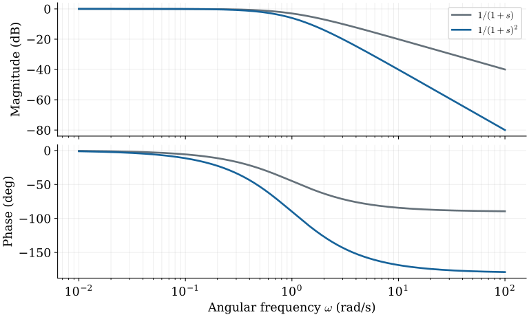
$$ 20\log_{10}|(j\omega+a)^m|=m\,20\log_{10}|j\omega+a|,\qquad \arg(j\omega+a)^m=m\tan^{-1}(\omega/a). $$

A double pole changes the high-frequency slope by $-40$ dB/decade and contributes $-180^\circ$ in total. Its approximate phase ramp has slope $-90^\circ$/decade across the two-decade transition. A repeated zero has the opposite signs. Multiplicity must be counted even when several break frequencies coincide.

A second-order denominator

Repeated real poles are one possible second-order factor, but a second-order denominator may also have complex conjugate poles. The distant magnitude limits remain simple; the behavior between them now depends strongly on damping. Write the denominator in terms of the natural frequency $\omega_n\gt 0$ and damping ratio $\zeta$.

$$ G(s)=\frac{1}{s^2+2\zeta\omega_n s+\omega_n^2},\qquad |G(j\omega)|=\frac{1}{\sqrt{(\omega_n^2-\omega^2)^2+(2\zeta\omega_n\omega)^2}}. $$

The low-frequency gain is $1/\omega_n^2$. At high frequency the magnitude approaches $1/\omega^2$, hence $-40$ dB/decade. At $\omega=\omega_n$, the magnitude is $1/(2\zeta\omega_n^2)$. Smaller positive damping produces a sharper amplification near the natural frequency. At $\zeta=1$, the denominator is $(s+\omega_n)^2$. The figure sets $\omega_n=1$; a numerator $\omega_n^2$ would normalize DC gain to one.

Locate the second-order poles

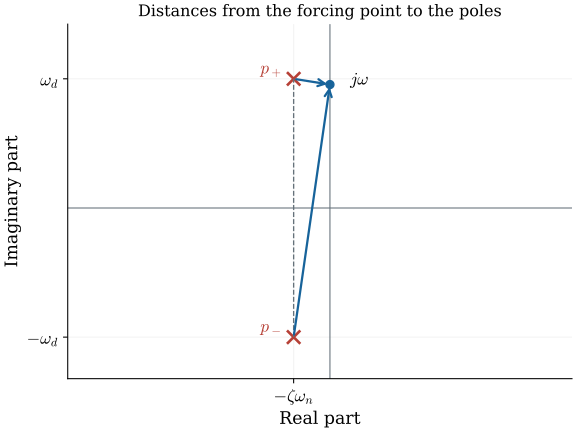
The pole locations explain this damping dependence geometrically. With unit numerator, the frequency-response magnitude is the reciprocal of the product of the distances from $j\omega$ to the two poles. A lightly damped pole lies close to the imaginary axis, so this product can become small near the natural frequency.

$$ \begin{aligned}s^2+2\zeta\omega_n s+\omega_n^2&=(s-p_+)(s-p_-),\\p_\pm&=-\zeta\omega_n\pm j\omega_n\sqrt{1-\zeta^2},\\|G(j\omega)|&=\frac1{|j\omega-p_+|\,|j\omega-p_-|}.\end{aligned} $$

For $0\lt \zeta\lt 1$, the roots form a complex conjugate pair. Evaluating at $j\omega$ measures the distance from that point to each pole. When damping is small, the upper pole approaches the imaginary axis near $j\omega_n$. One distance becomes small as the forcing frequency passes nearby, making the reciprocal product large. As $\zeta$ approaches one, the roots meet at $-\omega_n$ and the response becomes that of a repeated real pole.

Low, high, and natural-frequency limits

The geometric picture can be checked by evaluating three useful frequency regions. At low and high frequencies, one denominator term dominates. At the natural frequency, the real terms cancel and the damping term alone determines the magnitude.

$$ \begin{aligned}G(j\omega)&=\frac1{\omega_n^2-\omega^2+j2\zeta\omega_n\omega},\\\omega\ll\omega_n:&\quad |G|\approx1/\omega_n^2,\\\omega\gg\omega_n:&\quad |G|\approx1/\omega^2,\\\omega=\omega_n:&\quad |G|=1/(2\zeta\omega_n^2).\end{aligned} $$

The constant term controls the low-frequency limit, while the quadratic term controls the high-frequency limit. Thus the high-frequency logarithmic magnitude is $20\log_{10}(1/\omega^2)=-40\log_{10}\omega$, giving a $-40$ dB/decade slope. At the natural frequency the real denominator terms cancel; the damping term alone sets the magnitude. Smaller positive damping raises the response in this region without changing either far-frequency slope.

Resonance frequency and damped natural frequency

A large response near $\omega_n$ does not mean that the maximum occurs exactly there. Nor is the forcing frequency of maximum response generally equal to the damped oscillation frequency of the transient. Distinguishing these frequencies is necessary when interpreting a resonance peak.

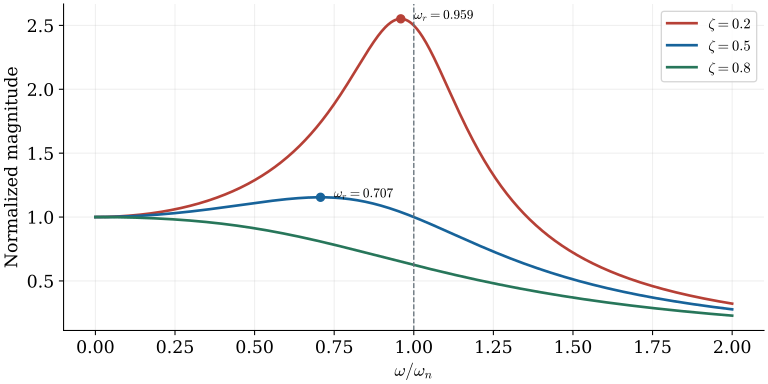
$$ \omega_r=\omega_n\sqrt{1-2\zeta^2},\quad 0\lt \zeta\lt \frac{1}{\sqrt{2}};\qquad \omega_d=\omega_n\sqrt{1-\zeta^2}. $$

Differentiate the squared magnitude denominator with respect to $\omega^2$ to obtain $\omega_r^2=\omega_n^2(1-2\zeta^2)$. A nonzero-frequency peak exists only when $\zeta\lt 1/\sqrt{2}$. For the DC-normalized second-order low-pass, the peak magnitude is $1/[2\zeta\sqrt{1-\zeta^2}]$. For the numerator-one model, divide this by $\omega_n^2$.

Find the resonant peak

To locate the peak precisely, minimize the squared magnitude of the denominator. Using $\omega^2$ as the independent variable reduces the calculation to a quadratic expression. The stationary point represents a nonzero-frequency resonance only when it lies in the positive-frequency range.

$$ \begin{aligned}x&=\omega^2,\\D(x)&=(\omega_n^2-x)^2+4\zeta^2\omega_n^2x,\\D^{\prime}(x)&=2(x-\omega_n^2)+4\zeta^2\omega_n^2,\\D^{\prime}(x)=0&\ \Longrightarrow\ x=\omega_n^2(1-2\zeta^2).\end{aligned} $$

Maximizing $|G|$ is equivalent to minimizing its squared denominator. A peak at a positive frequency exists only if $1-2\zeta^2\gt 0$. Substitution gives $|G(j\omega_r)|=1/[2\zeta\omega_n^2\sqrt{1-\zeta^2}]$. The imaginary part of a free-response pole is instead $\omega_d=\omega_n\sqrt{1-\zeta^2}$. The forced-response peak and the transient oscillation frequency answer different questions.

Phase of the complex pole pair

The second-order description is completed by its phase. The same damping term that controls amplification near resonance also controls how rapidly the denominator angle changes. A quadrant-aware angle calculation is essential once the real part of the denominator becomes negative.

$$ \phi(\omega)=-\operatorname{atan2}(2\zeta\omega_n\omega,\,\omega_n^2-\omega^2). $$

For positive damping, the phase is $-90^\circ$ exactly at $\omega_n$. Use the two-argument arctangent to preserve the correct quadrant above the natural frequency. As damping decreases, both the magnitude peak and the phase transition become sharper. At zero damping the transfer function has imaginary-axis poles and the usual stable steady-state interpretation at resonance fails.

Perspective

The same addition rules handle separated and repeated real factors, while the second-order form describes a complex pole pair. The distant slopes reveal the number of poles and zeros; damping determines the response near resonance. When interpreting a peak, distinguish the forcing frequency $\omega_r$ from the free-response frequency $\omega_d$, and retain the correct constant gain when normalizing the transfer function.

The next lecture uses these frequency-response ideas to assess dominant modes and model approximations in compensated systems.

References

Norman S. Nise, Control Systems Engineering, 6th ed., Wiley, 2011.

• §10.2: Bode construction and second-order factors.
• §10.8: Resonance and transient response.
• §§11.3–11.4: Lag and lead compensation.