Lecture 6: First- and Second-Order Systems
The review lectures gave us transfer functions and a way to invert them. We now start the analysis part of the course. The question is this: given a transfer function, what does the response look like, and how can we tell without computing it in full? The answer is built around poles and zeros. This lecture defines them, studies the two simplest building blocks, first- and second-order systems, and takes a short detour into the number $e$ that governs all of their responses.
Forced and natural responses
The total response of a system splits into two parts:
$$\text{total response} = \text{forced response} + \text{natural response}.$$The forced response is driven by the input. The natural response comes from the initial conditions (the system’s stored energy) and describes how the system behaves on its own. We saw both in Lecture 5: in $y(t) = e^{-at}y_0 + \frac ba(1 - e^{-at})$, the first term is natural and the second is forced.
To guess quickly whether a response is stable, unstable or oscillating, we look at the poles and zeros. When there is no time delay, the poles alone determine stability.
Poles and zeros
Let $G(s) = N(s)/D(s)$.
- Poles are the values of $s$ that make the transfer function infinite, that is, the roots of $D(s) = 0$. They are marked “$\times$” in the complex $s$-plane ($s = \sigma + j\omega$).
- Zeros are the values of $s$ that make the transfer function zero, that is, the roots of $N(s) = 0$. They are marked “$\circ$”.
For example, if $G(s) = N(s)/\big((s+p_1)(s+p_2)\cdots(s+p_n)\big)$, the poles are $-p_1, -p_2, \ldots, -p_n$, and $G(s)\to\infty$ as $s\to-p_i$.
A few additional facts:
- The system is asymptotically stable if and only if all poles have negative real parts, that is, all poles lie in the open left half-plane (LHP). Lecture 10 develops stability in detail.
- Zeros do not affect stability, but they change the amplitude and speed of the response (Lecture 9).
- Common roots of $N$ and $D$ cancel. The cancellation must be taken into account when listing the poles and zeros that actually shape the input-output response.
Example 1. Find the poles and zeros of
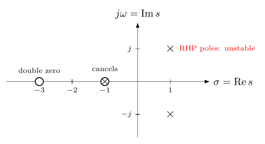
$$G(s) = \frac{(s+1)(s+3)(s+3)}{(s+1)(s-1+j)(s-1-j)} .$$Before cancellation, the zeros are $-1$, $-3$, $-3$ and the poles are $-1$ and $1\pm j$. The factor $(s+1)$ cancels, which leaves a double zero at $-3$ and a complex-conjugate pair of poles at $1\pm j$. Those poles have positive real parts, so the system is unstable.
Example 2. Find the poles and zeros of the system described by
$$\ddot x + 2\dot x + 1 = 2\dot u,$$where $x(t)$ is the output and $u(t)$ is the input, with zero initial conditions. The transfer function describes only how the input $u$ reaches the output. Taking Laplace transforms,
$$s^2X(s) + 2sX(s) + \frac1s = 2sU(s) \quad\Longrightarrow\quad X(s) = \underbrace{\frac{2s}{s(s+2)}}_{G(s)}\,U(s) - \frac{1}{s^2(s+2)} .$$Note that the constant term $1$ transforms to $1/s$, not $1$. It acts as a constant input and adds its own term to the response, but it does not change $G(s)$. The transfer function $G(s) = 2s/(s(s+2))$ has poles at $0$ and $-2$ and a zero at $0$. The zero cancels the pole at the origin, leaving $G(s) = 2/(s+2)$. (If the equation was meant to read $\ddot x + 2\dot x + x = 2\dot u$, then $G(s) = 2s/(s+1)^2$, with a double pole at $-1$ and a zero at $0$.)
First-order systems
A first-order differential equation gives a first-order system, and its response is an exponential decay or growth.
Demo: pushing a block against friction. A block of mass $m$ slides on a surface with viscous friction force $f_dv$. With the applied force $f$ as the input and the velocity $v$ as the output, Newton’s law gives
$$m\dot v = -f_dv + f \quad\Longrightarrow\quad \frac{V(s)}{F(s)} = \frac{1/m}{s + f_d/m} .$$The single pole is at $s = -f_d/m$.
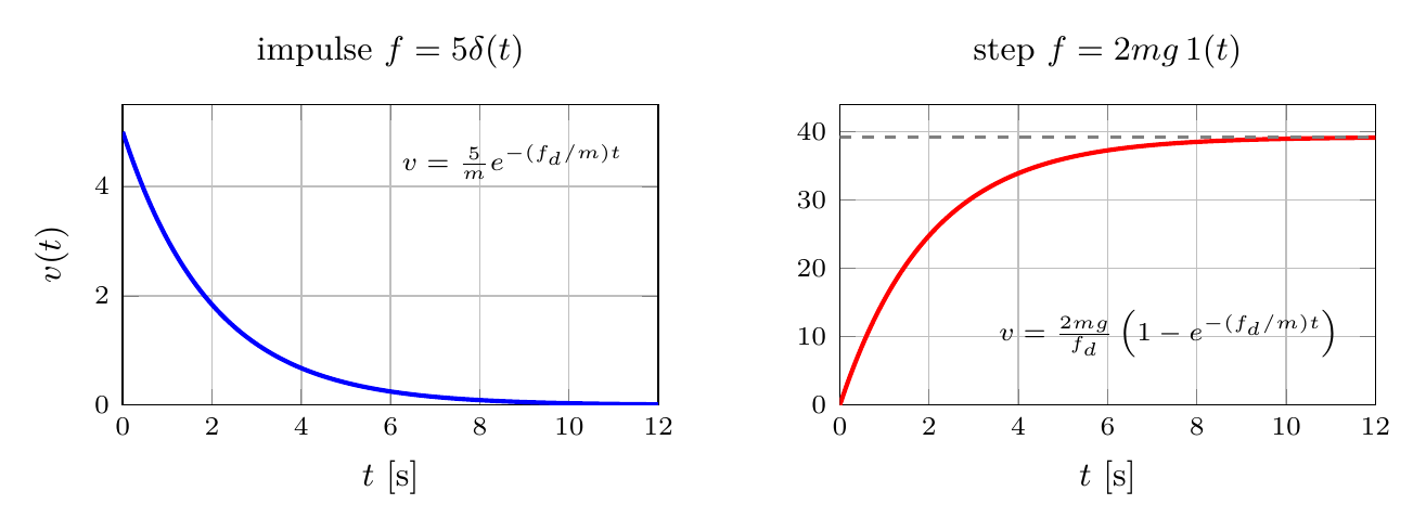
- A sharp hit. An impulse $f = 5\delta(t)$ gives $F(s) = 5$ and $v(t) = \mathcal{L}^{-1}\left\{\frac{5/m}{s + f_d/m}\right\} = \frac5m e^{-(f_d/m)t}$: the block jumps to speed $5/m$ and coasts to a stop.
- A continuous push. A step $f = 2mg\,1(t)$ gives $V(s) = \frac{1/m}{s+f_d/m}\cdot\frac{2mg}{s} = \frac{K_1}{s} + \frac{K_2}{s+f_d/m}$ with $K_1 = \lim_{s\to0}sV(s) = 2mg/f_d$ and $K_2 = -2mg/f_d$, so $v(t) = \frac{2mg}{f_d}\left(1 - e^{-(f_d/m)t}\right)$: the block accelerates until friction balances the push.
The generalized first-order system. Every first-order system has the form
$$G(s) = \frac{b}{s+a} .$$With zero initial conditions and a unit step input $U(s) = 1/s$,
$$Y(s) = \frac{b}{s(s+a)} = \frac{b/a}{s} - \frac{b/a}{s+a} \quad\Longrightarrow\quad y(t) = \frac ba\left(1 - e^{-at}\right).$$The term $-\frac ba e^{-at}$ is the transient, which comes from the pole; $\frac ba$ is the steady-state value, the DC gain of Lecture 5.
- The response decays to steady state (stable) when the pole $-a$ satisfies $\mathrm{Re}(\text{pole}) \lt 0$.
- It grows without bound (unstable) when $\mathrm{Re}(\text{pole}) \gt 0$.
The location of the pole dictates stability, and the value of the pole dictates how fast the response decays or grows.
For a stable first-order system, three performance measures follow directly from $1 - e^{-at}$:
- Time constant $\tau = 1/a$: the time for the step response to reach 63% of the final value.
- Rise time $T_r = 2.2/a$: the time to go from 10% to 90% of the final value ($\ln 9 = 2.197$).
- Settling time $T_s = 4/a$: the time to reach and stay within 2% of the final value.
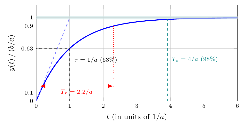
The dashed line in the figure is the initial slope: the response would reach its final value in one time constant if it kept its initial rate.
About $e$
Why do “63%” and “4 time constants” appear? Both come from the number $e = 2.71828\ldots$, which is worth a short detour.
Exponential growth in nature. A population with unlimited resources grows at a rate proportional to its size,
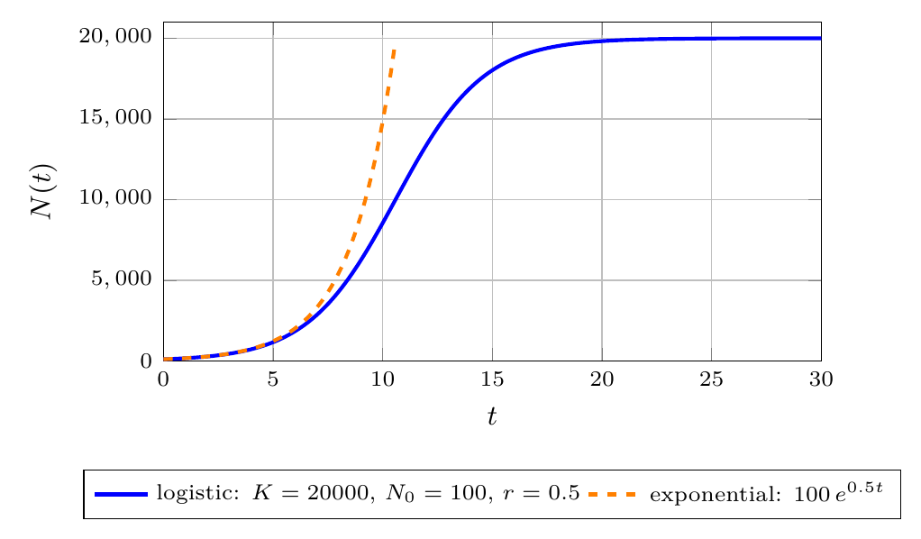
$$\frac{dN}{dt} = \underbrace{(\text{birth rate} - \text{death rate})}_{r}\,N \quad\Longrightarrow\quad N(t) = e^{rt}N(0).$$This is a first-order system with a pole at $s = r \gt 0$: an unstable one. In reality, resources are limited. The logistic growth model slows the growth as $N$ approaches a carrying capacity $K$:
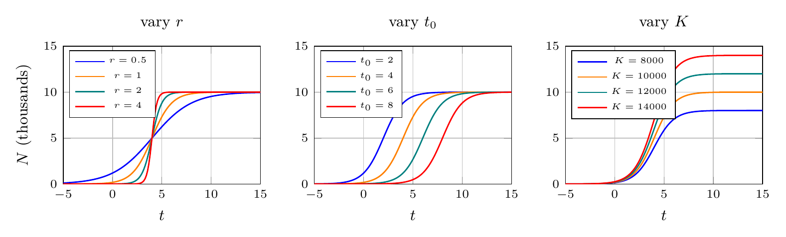
$$\frac{dN}{dt} = r\frac{K-N}{K}N \quad\Longrightarrow\quad N(t) = \frac{KN_0e^{rt}}{(K-N_0) + N_0e^{rt}} = \frac{K}{1 + \frac{K-N_0}{N_0}e^{-rt}} .$$At first the two models agree; then the logistic curve bends over and levels off at $K$.
The logistic S curve. The logistic solution can be written as
$$N(t) = \frac{K}{1 + e^{-r(t-t_0)}},$$where $K$ is the final value, $r$ the logistic growth rate, and $t_0$ the midpoint. Each parameter changes the curve in a distinct way:
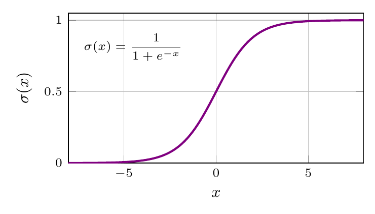
Sigmoid as a neural-network activation. The normalized logistic curve is
$$\sigma(x) = \frac{1}{1+e^{-x}}.$$A neuron first forms a weighted sum $z = \mathbf{w}^{\mathsf T}\mathbf{h}+b$ of its inputs, then applies an activation function, $a = f(z)$. A nonlinear activation lets a network represent nonlinear relationships; stacking affine layers without it would still give an affine map. Sigmoid was widely used in early neural networks because it is smooth and maps any real input into $(0,1)$. At a binary-classification output, $\sigma(z)$ represents the model’s estimate of $P(y=1\mid\mathbf{h})$. A hidden neuron’s sigmoid output need not have a probability interpretation. The exponential $e^{-z}$ creates the S shape and its saturation at both ends.
Training uses backpropagation, which multiplies derivatives along a chain of layers. For sigmoid,
$$\sigma'(z) = \frac{e^{-z}}{(1+e^{-z})^2} = \sigma(z)\bigl(1-\sigma(z)\bigr) \le \frac14.$$The derivative approaches zero for large positive or negative $z$. These small factors can make learning signals shrink through many hidden layers: the vanishing-gradient problem. Sigmoid remains useful for binary outputs and gates, but this saturation motivated other hidden-layer activations (Goodfellow, Bengio and Courville, Chapter 6).
From sigmoid to ReLU, ELU and SELU. One influential development was the rectified linear unit, $\operatorname{ReLU}(z)=\max(0,z)$. Its positive branch is linear, with derivative 1, so it avoids sigmoid’s positive-side saturation. ReLU contains no exponential, but its negative branch has zero derivative. The exponential linear unit (ELU), introduced in 2015, retains the linear positive branch and adds a negative branch $\alpha(e^z-1)$, with $\alpha\gt 0$. Negative outputs help bring mean activations closer to zero. Here the exponential returns, shaping a branch that approaches $-\alpha$ as $z\to-\infty$ (Clevert, Unterthiner and Hochreiter, 2015/2016).
The scaled exponential linear unit (SELU), introduced in 2017, builds on ELU:
$$\operatorname{SELU}(z) = \lambda \begin{cases} z, & z\gt 0,\\ \alpha(e^z-1), & z\le0, \end{cases} \qquad \alpha\approx1.6733,\quad\lambda\approx1.0507.$$Its positive slope is $\lambda\gt 1$; its negative branch tends to $-\lambda\alpha$ and has derivative $\lambda\alpha e^z$ for $z\lt 0$. Thus SELU still saturates for very negative inputs. The chosen constants balance these branches so that, under the assumptions of self-normalizing neural networks, activation means and variances are driven toward zero and one as they pass through layers (Klambauer et al., 2017).
This property depends on the network setup: standardized inputs, suitable feedforward layers, LeCun-normal weight initialization (variance $1/n_{\mathrm{in}}$), and AlphaDropout if dropout is used. It is not guaranteed by selecting SELU alone; see the Keras SELU documentation. SELU is a later specialized development, rather than a universal replacement for sigmoid or ReLU.
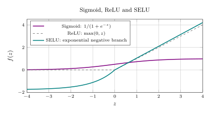
Where is $e$? In sigmoid, $e^{-z}$ creates a bounded S curve. In ELU and SELU, $e^z-1$ creates negative saturation while the positive branch stays linear. In our control responses, $e^{at}$ sets growth or decay in time. The same exponential function shapes all three, although a neural activation is a static input-output map and a system response evolves with time.
What is $e$? The Taylor expansion
$$e^x = 1 + \frac{x}{1!} + \frac{x^2}{2!} + \cdots + \frac{x^n}{n!} + \cdots$$with $x = 1$ gives
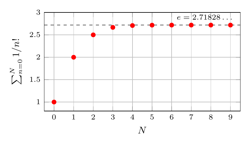
$$e = \sum_{n=0}^\infty\frac{1}{n!} = 2.71828\ldots$$The partial sums converge very quickly:
import math
print(math.e)
for ii in range(10):
    print(sum(1 / math.factorial(k) for k in range(ii)))
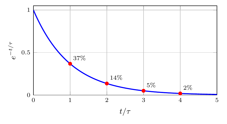
Solution concepts of $e^{at}x(0)$. The natural response of $\dot x = ax$ is $e^{at}x(0)$. When $a\lt 0$, define the time constant $\tau \triangleq 1/|a|$. Four numbers are worth memorizing:
$$e^{-1}\approx37\%, \qquad e^{-2}\approx14\%, \qquad e^{-3}\approx5\%, \qquad e^{-4}\approx2\%.$$After $3\tau$ the transient has decayed to about 5% of its initial size and has approximately converged; after $4\tau$ it is within 2%. This is where $T_s = 4/a$ comes from, and the 63% of the time constant is $1 - e^{-1}$. For the step input, when $a\lt 0$ and $u(t) = 1(t)$, the solution of $\dot x = ax + bu$ with $x(0)=0$ is $x(t) = \frac{b}{|a|}\left(1 - e^{at}\right)$.
Pole locations and the response
The first-order case generalizes. Each pole $\lambda$ contributes a term $e^{\lambda t}$ to the natural response. For a real pole the term is a pure exponential. For a complex pole $\lambda = \sigma + j\omega$, Euler’s formula gives
$$e^{\lambda t} = e^{(\sigma+j\omega)t} = e^{\sigma t}e^{j\omega t} = e^{\sigma t}(\cos\omega t + j\sin\omega t).$$Complex poles of a real system come in conjugate pairs, and the imaginary parts combine into a real oscillation $e^{\sigma t}\cos(\omega t + \phi)$. The real part $\sigma$ sets the envelope and the imaginary part $\omega$ sets the oscillation frequency. This gives a map from pole location to response shape:
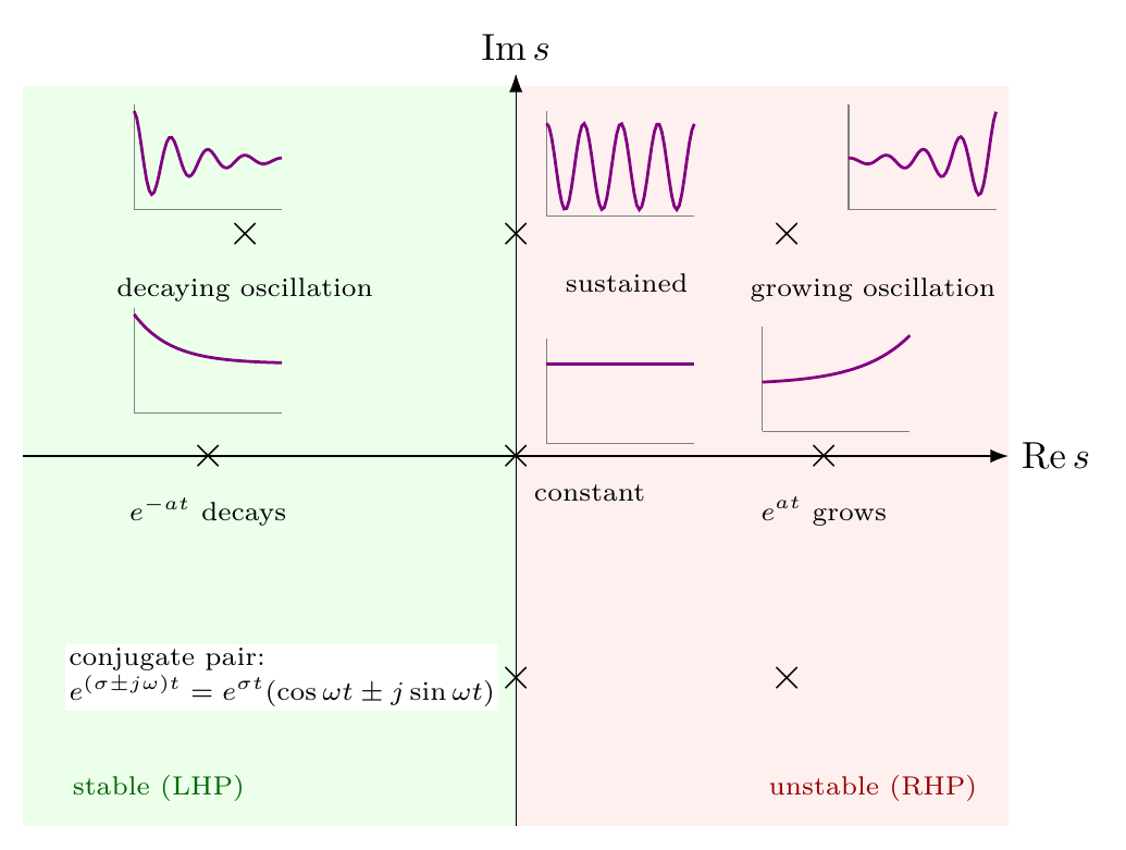
- Real pole in the LHP ($\lambda\in\mathbb{R}$, $\lambda\lt 0$): exponential decay.
- Pole at the origin: a constant.
- Real pole in the RHP: exponential growth.
- Complex pair in the LHP: decaying oscillation.
- Pair on the imaginary axis ($\lambda = \pm j\omega$): sustained, bounded oscillation.
- Complex pair in the RHP: growing oscillation.
Moving left speeds up the decay; moving up or down raises the oscillation frequency.
Second-order systems
A second-order differential equation gives a second-order system. Its response has an exponential decay or growth and possibly an oscillation. The mass-spring-damper of Lecture 3 is the standard example:
$$m\ddot x(t) + b\dot x(t) + kx(t) = f(t).$$Transforming with zero initial conditions,
$$ms^2X(s) + bsX(s) + kX(s) = F(s) \quad\Longrightarrow\quad \frac{X(s)}{F(s)} = \frac{1/m}{s^2 + \frac bms + \frac km}.$$If the velocity is the output instead, multiplying by $s$ (differentiation in time) gives $\frac{sX(s)}{F(s)} = \frac{s/m}{s^2 + \frac bms + \frac km}$. The denominator, and so the poles, is the same; only a zero at the origin is added.
The generalized second-order system. We write
$$G(s) = \frac{b_0}{s^2 + a_1s + a_0} = k\,\frac{\omega_n^2}{s^2 + 2\zeta\omega_ns + \omega_n^2},$$where $k$ is the DC gain and
- $\omega_n$ is the natural frequency, the frequency of oscillation without damping;
- $\zeta$ is the damping ratio, $\zeta = \dfrac{\text{exponential decay frequency}}{\text{natural frequency}} = \dfrac{\zeta\omega_n}{\omega_n}$;
- $\omega_d = \omega_n\sqrt{1-\zeta^2}$ is the damped frequency of oscillation, defined for $0\lt \zeta\lt 1$.
For the mass-spring-damper, $\omega_n = \sqrt{k/m}$ and $\zeta = b/(2\sqrt{km})$.
Poles. The roots of $s^2 + 2\zeta\omega_ns + \omega_n^2$ are
$$p_{1,2} = -\zeta\omega_n \pm \omega_n\sqrt{\zeta^2-1} \qquad (\zeta\ge1),$$$$p_{1,2} = -\zeta\omega_n \pm j\omega_n\sqrt{1-\zeta^2} = -\zeta\omega_n \pm j\omega_d \qquad (0\le\zeta\lt 1).$$
Four cases. For a unit step input,
$$Y(s) = G(s)U(s) = \frac{k\omega_n^2}{s^2 + 2\zeta\omega_ns + \omega_n^2}\cdot\frac1s,$$and the damping ratio determines which of four responses we get.
- Overdamped, $\zeta\gt 1$. Two distinct real poles $p_{1,2} = -\zeta\omega_n\pm\omega_n\sqrt{\zeta^2-1}$. Natural response $c_1e^{p_1t} + c_2e^{p_2t}$: a sluggish approach with no overshoot, dominated by the slower pole.
- Underdamped, $0\lt \zeta\lt 1$. A complex-conjugate pair $p_{1,2} = -\zeta\omega_n\pm j\omega_d$. Natural response $c_1e^{-\zeta\omega_nt}\cos(\omega_dt + \phi)$: an oscillation at the damped frequency $\omega_d$, with phase shift $\phi$, inside a decaying envelope.
- Undamped, $\zeta=0$. Imaginary poles $p_{1,2} = \pm j\omega_n$. Natural response $c_1\cos(\omega_nt + \phi)$: an oscillation that never decays.
- Critically damped, $\zeta=1$. A repeated real pole $p_{1,2} = -\omega_n$. Natural response $c_1te^{-\omega_nt} + c_2e^{-\omega_nt}$: the fastest response without overshoot.
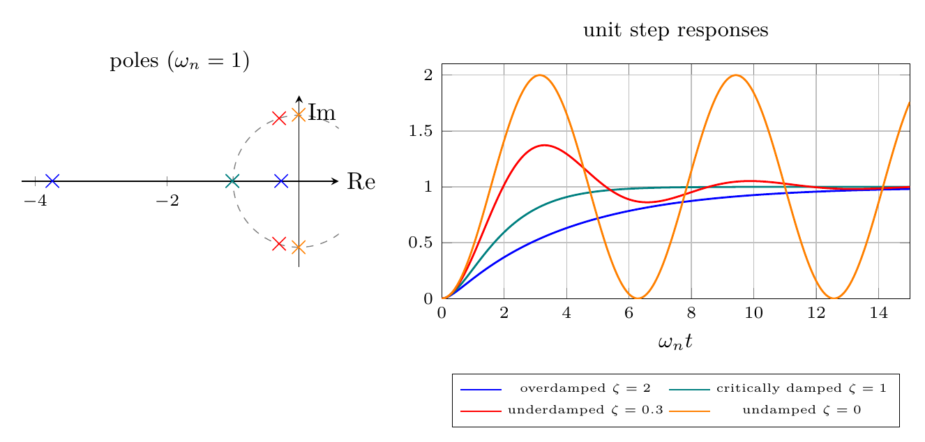
As $\zeta$ decreases from 2 to 0, the poles move from the real axis (overdamped), meet at $-\omega_n$ (critically damped), split onto a circle of radius $\omega_n$ (underdamped) and reach the imaginary axis (undamped). The step responses go from sluggish to oscillatory accordingly.
Summary and outlook
- Total response = forced response + natural response. Poles ($\times$) are roots of the denominator, zeros ($\circ$) roots of the numerator; poles decide stability.
- First-order systems $b/(s+a)$: $y = \frac ba(1-e^{-at})$, with $\tau = 1/a$, $T_r = 2.2/a$, $T_s = 4/a$.
- $e^{-1}, e^{-2}, e^{-3}, e^{-4}\approx 37\%, 14\%, 5\%, 2\%$. Exponentials also describe population growth; sigmoid uses $e^{-z}$ for a bounded activation, while ELU and SELU use $e^z-1$ for a saturating negative branch and retain a linear positive branch.
- Each pole contributes $e^{\lambda t}$: the real part sets decay or growth, the imaginary part sets oscillation.
- Second-order systems $k\omega_n^2/(s^2+2\zeta\omega_ns+\omega_n^2)$ are overdamped, critically damped, underdamped or undamped depending on $\zeta$.
The underdamped case is the most important in practice, because most well-tuned control loops behave this way. The next lecture derives its step response exactly and turns it into design specifications: peak time, overshoot and settling time.
References
-
N. S. Nise, Control Systems Engineering, 6th ed.: §4.1 Introduction (p. 162); §4.2 Poles, Zeros, and System Response (p. 162); §4.3 First-Order Systems (p. 166); §4.4 Second-Order Systems: Introduction (p. 168); §4.5 The General Second-Order System (p. 173).
-
X. Chen and M. Tomizuka, Introduction to Modern Controls, with Illustrations in MATLAB and Python: §6.1.1 The Solution to $\dot x = ax + bu$ (p. 103); §6.1.2 The Irrational Number $e$ (p. 105); §8.2.1 Method of Eigenvalue Locations (p. 144).
-
I. Goodfellow, Y. Bengio and A. Courville, Deep Learning (2016): Chapter 6, Deep Feedforward Networks, §§6.2.2.2 and 6.3 (online chapter).
-
D.-A. Clevert, T. Unterthiner and S. Hochreiter, Fast and Accurate Deep Network Learning by Exponential Linear Units (ELUs), preprint 2015, ICLR 2016 (paper).
-
G. Klambauer, T. Unterthiner, A. Mayr and S. Hochreiter, Self-Normalizing Neural Networks, NeurIPS 2017 (paper).