Lecture 11: PD Control of an Unstable System
The previous lectures analyzed given transfer functions, and Lecture 10 gave a test for stability. With this lecture we move from analysis to design. We close a feedback loop around a plant and ask how to choose the controller so that the closed loop is stable. The main tool is the Routh array of Lecture 10, which turns stability into simple inequalities on the design parameters without solving for any roots. We apply it to two second-order plants, one open-loop stable and one open-loop unstable, and discover why derivative action is so valuable.
Throughout, the plant $G$ and controller $C$ sit in a unity negative-feedback loop. By the single-loop rule of Lecture 2,

The closed-loop poles are the roots of $1 + CG = 0$.
An open-loop stable plant
Take $C = 1$ and
$$G_1(s) = \frac{K}{(s+1)^2},\qquad \frac{Y}{U} = \frac{K}{(s+1)^2 + K} = \frac{K}{s^2 + 2s + (1+K)}.$$The Routh array of the characteristic polynomial is
| $s^2$ | $1$ | $1+K$ |
| $s^1$ | $2$ | $0$ |
| $s^0$ | $1+K$ |
The closed loop is stable exactly when the first column has no sign changes, that is, when $1 + K \gt 0$, or $K \gt -1$.
What does this mean physically? The DC gain of the plant is $G_1(0) = K$. Physical systems are usually built with a positive DC gain: a positive voltage should turn a motor in the positive direction. So $K\gt 0$, and the closed loop is automatically stable. An open-loop stable plant under negative feedback is usually easy to keep stable. The same workflow applies unchanged to higher-order plants, and at no point do we need to solve for the roots.
An open-loop unstable plant
The situation changes when the plant itself is unstable. Take $C=1$ and
$$G_2(s) = \frac{K}{(s-1)(s+1)} = \frac{K}{s^2 - 1},\qquad \frac{Y}{U} = \frac{K}{s^2 + (K - 1)}.$$The $s^1$ coefficient is zero, so the Routh array breaks down (one could replace the zero by a small $\epsilon$). Here the roots are easy to read directly from $s^2 = 1 - K$:
| Gain | Closed-loop poles | Stability |
|---|---|---|
| $K \lt 1$ | $s = \pm\sqrt{1-K}$ (one in the RHP) | unstable |
| $K = 1$ | double pole at $s = 0$ | unstable |
| $K \gt 1$ | $s = \pm j\sqrt{K-1}$ | marginally stable |
As $K$ increases, the two closed-loop poles move toward each other along the real axis, meet at the origin and then travel up and down the imaginary axis:
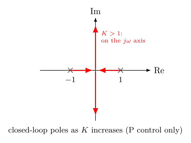
With a single constant gain, strict stability is impossible. The best achievable is marginal stability, a sustained oscillation. The plant needs more than proportional control.
Adding derivative action
Why does proportional control fail? The characteristic polynomial $s^2 + (K-1)$ has no $s^1$ term, so there is nothing to provide damping. A derivative term supplies exactly that. With the PD controller $C(s) = K_p + K_d s$,
$$\frac{Y}{U} = \frac{K(K_p + K_d s)}{s^2 - 1 + K(K_p + K_d s)} = \frac{K(K_p + K_d s)}{s^2 + KK_d\,s + (KK_p - 1)}.$$The Routh array is now
| $s^2$ | $1$ | $KK_p - 1$ |
| $s^1$ | $KK_d$ | $0$ |
| $s^0$ | $KK_p - 1$ |
and the closed loop is stable if and only if
$$KK_d \gt 0 \quad\text{and}\quad KK_p \gt 1.$$For $K\gt 0$ this means any positive derivative gain together with a proportional gain above $1/K$.
This result is striking. P control alone at best reaches the imaginary axis; adding even a small derivative gain moves the poles into the open left half-plane and makes the loop strictly stable.
Summary and outlook
- Closed-loop poles are the roots of $1 + CG = 0$, and the Routh array turns stability into inequalities on the gains.
- An open-loop stable plant with a positive DC gain stays stable under negative proportional feedback.
- An open-loop unstable second-order plant cannot be strictly stabilized by P control. PD control stabilizes it when $KK_d \gt 0$ and $KK_p \gt 1$.
Stability is the first requirement of any design, but not the last. Once the loop is stable, we want the output to follow the reference accurately. Lecture 12 quantifies how accurately, through the steady-state error.
References
- N. S. Nise, Control Systems Engineering, 6th ed.: §6.2 Routh-Hurwitz Criterion (p. 305); §6.4 Routh-Hurwitz Criterion: Additional Examples (p. 314); §9.3 Improving Transient Response via Cascade Compensation (p. 469), on PD control.
- X. Chen and M. Tomizuka, Introduction to Modern Controls, with Illustrations in MATLAB and Python: §8.2.2 Routh-Hurwitz Criterion for Continuous-Time LTI Systems (p. 146).