Lecture 2: Block Diagram Simplification

Lecture 1 showed feedback loops informally. To analyze them, we need a precise way to describe how signals flow between components. The textbook feedback loop, with one controller $C$, one plant $P$ and unity feedback, is easy to analyze. Practical controllers are rarely that simple: they contain extra loops, feedforward branches and summing junctions in awkward places. The goal of this lecture is a small set of rules that reduces any interconnection of blocks to a single equivalent transfer function from input to output. Once we have that single function, every analysis tool in the following lectures applies.

Throughout, we consider linear systems and work only with transfer functions in the Laplace domain. Signals are written in capitals, for example $Y(s)$, and the argument $(s)$ is often omitted.

The basic elements

Every block diagram is built from three elements. The first is the block: a signal enters, and the output is the transfer function times the input.

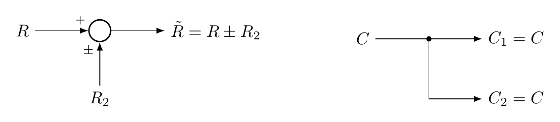
Real systems combine several signals, which the second element handles. A summing junction adds its incoming signals, each carrying the sign ($+$ or $-$) written near its arrowhead; the outgoing signal is the signed sum. Some textbooks draw a cross inside the circle; we use a plain circle. The third element, the pickoff point, is a dot where one signal is copied into several branches. Every branch carries exactly the same signal.

Series and parallel connections

With these elements we can build the two simplest interconnections. In a series connection the output of one block feeds the next, so we just apply the block rule twice:

$$C(s) = G_2(s)\,G_1(s)\,R(s).$$

Notice the order in which we wrote the product: the input comes last, and the blocks appear from right to left in the order the signal meets them. For single-input single-output systems the order does not matter, because scalar multiplication commutes. For multivariable (MIMO) systems the blocks are matrices, and this convention becomes essential, so it is worth adopting now.

In a parallel connection, a pickoff point sends one signal through several channels whose outputs are summed:

$$C = G_1R + G_2R + G_3R = (G_1 + G_2 + G_3)\,R.$$

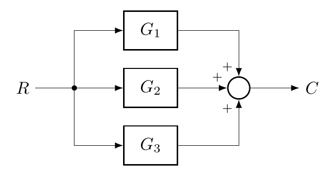
In short, series blocks multiply and parallel blocks add.

The feedback loop

The third fundamental structure, and the reason for this course, is the feedback loop:

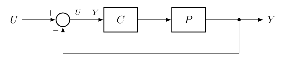
We find its transfer function the same way as before, by tracing the signals. After the summing junction the signal is $U - Y$. After the controller it is $C(U-Y)$, and after the plant it is $PC(U-Y)$. Because of the pickoff point, that last signal is the output $Y$. So

$$Y = PC\,(U - Y).$$

Collecting the $Y$ terms on the left gives $(1 + PC)\,Y = PC\,U$, and therefore

$$\frac{Y}{U} = \frac{PC}{1 + PC}.$$

Experienced control engineers rarely repeat this algebra; they read the result directly from the diagram. Follow the input: part of it travels the direct (forward) path, through $C$ and $P$, and supplies the numerator $PC$. The feedback creates the denominator, which is one plus the product of all blocks around the loop. For a single loop,

$$\frac{Y}{U} = \frac{\text{product of blocks on the forward path}}{1 \pm \text{product of all blocks around the loop}},$$

with $1 +$ for negative feedback and $1 -$ for positive feedback.

As an exercise, apply this rule to two variations. With positive feedback the result is $\dfrac{PC}{1-PC}$. With an additional block $H$ in the feedback path, the forward path is still $PC$, but the loop now contains $P$, $C$ and $H$:

Moving summing junctions and pickoff points

The single-loop rule is powerful, but practical diagrams often have loops that overlap or branches that leave from inside a loop. To untangle them, we need to move summing junctions and pickoff points across blocks without changing any signal. Each move is paid for by inserting a compensating block.

Moving a summing junction ahead of a block. Originally $E = G_1U + Y$. If we move the junction in front of $G_1$, the $U$ channel still passes through $G_1$, so the $Y$ channel would be multiplied by $G_1$ too, unless we first pass it through $1/G_1$:

Check: $E = G_1\bigl(U + \tfrac{1}{G_1}Y\bigr) = G_1U + Y$, as before.

Moving a pickoff point past a block. Originally the branch carries $U$. If we pick the signal off after $G_1$, where it has become $G_1U$, the branch must undo that gain:

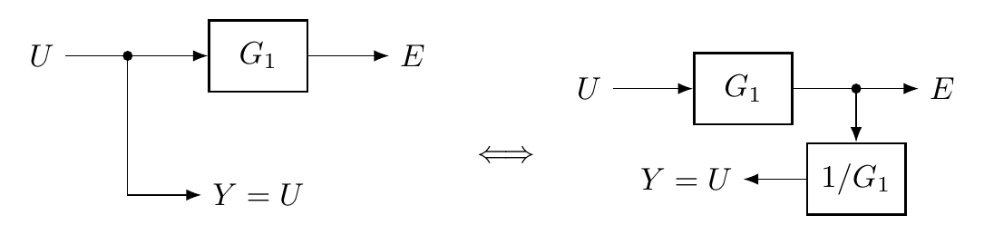
In both cases the compensating block on the side branch is $1/G$. With the single-loop rule and these two moves, we can reduce surprisingly complex diagrams, as the next example shows.

A worked example

Consider the following diagram. There is a local positive-feedback loop around $G_1$, and the signal $E$ (taken before $G_1$) is also sent forward into two later summing junctions:

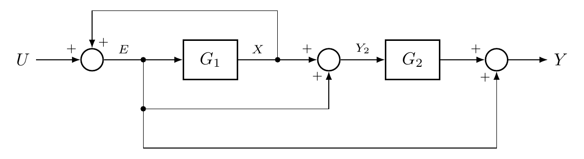
Its equations are $E = U + X$, $X = G_1E$, $Y_2 = X + E$ and $Y = G_2Y_2 + E$. We could solve them directly, but the goal is to see how the graphical rules lead to the answer.

Step 1: isolate the local loop. The difficulty is that $E$ is picked off inside the loop, so the loop is not self-contained. Moving that pickoff past $G_1$ to the loop output $X$ fixes this; by the rule above, the branch now needs $1/G_1$ (since $X/G_1 = E$). The loop stands alone, and because the feedback is positive,

$$\frac{X}{U} = \frac{G_1}{1 - G_1}.$$

Step 2: create clean parallel paths. The branch carrying $E$ still splits into two junctions. Instead, we pick off $X$ twice, giving each branch its own $1/G_1$:

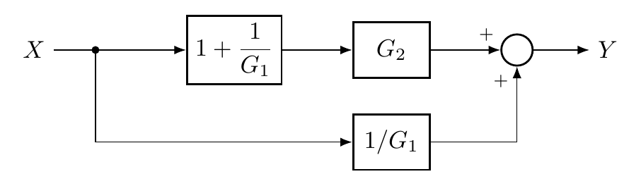
The first junction now adds $X$ and $X/G_1$, two parallel paths, which gives $1 + 1/G_1$. From $X$ to $Y$ there are then two parallel paths:

$$\frac{Y}{X} = \frac{1}{G_1} + G_2\left(1 + \frac{1}{G_1}\right).$$

Step 3: combine in series. The two results are in series:

$$\frac{Y}{U} = \left[\frac{1}{G_1} + G_2\left(1 + \frac{1}{G_1}\right)\right]\frac{G_1}{1 - G_1} = \frac{1 + G_2(1 + G_1)}{1 - G_1}.$$

Solving the original equations directly gives the same result: $E = U/(1-G_1)$ and $Y = G_2(G_1 + 1)E + E$. A diagram that looked cumbersome has become two blocks in series.

Summary and outlook

• A pickoff point means “same signal”; a summing junction means “signed sum”.
• Series blocks multiply (input last, blocks in signal order); parallel blocks add.
• A single loop gives forward path $/\,(1 \pm$ loop product$)$, with $+$ for negative feedback.
• To untangle a diagram, move junctions and pickoff points until each loop stands alone and the branches form clean parallel paths, then reduce from the inside out.

We can now reduce any linear interconnection to one transfer function. Two questions remain before we can analyze a loop: where do the transfer functions inside the blocks come from, and what do they tell us about the time response? The next lecture takes up the first question, the modeling of dynamic systems; Lectures 4 and 5 then review the Laplace transform that connects models to transfer functions.

References

• N. S. Nise, Control Systems Engineering, 6th ed.: §5.1 Introduction (p. 236); §5.2 Block Diagrams (p. 236); §5.3 Analysis and Design of Feedback Systems (p. 245).
• X. Chen and M. Tomizuka, Introduction to Modern Controls, with Illustrations in MATLAB and Python: §3.3 From Laplace Transform to Transfer Functions (p. 41).