Lecture 12: Steady-State Error
A stable closed loop is necessary, but it is not enough: we also want the output to follow the reference. This lecture asks how closely a unity-feedback loop tracks three standard references (a step, a ramp and a parabola) once the transients have died out. The answer depends on a single structural property of the loop, its type, and it leads directly to a first gain-design problem.
Error and sensitivity
We work with the standard loop and three test references:
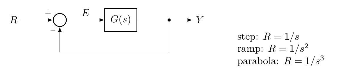
The error is the difference between reference and output. Using the single-loop rule for $Y$,
$$E = R - Y = R - \frac{G}{1+G}R = \frac{1}{1+G}\,R.$$The factor multiplying $R$ is so important that it has a name, the sensitivity function
$$S(s) = \frac{1}{1+G(s)}.$$It measures how sensitive the error is to the reference; when $|S|$ is small, the tracking error is small. Its complement,
$$T(s) = 1 - S(s) = \frac{G}{1+G},$$is the complementary sensitivity function, which is simply the reference-to-output transfer function. The pair $S$ and $T$ appears throughout advanced control.
System type
How large the error becomes depends on the behavior of $G$ near $s = 0$. To expose it, factor out all poles at the origin:
$$G(s) = \frac{b_m s^m + \dots + b_1 s + b_0}{s^{\alpha}\,(a_n s^n + \dots + a_1 s + a_0)},\qquad a_0, b_0 \neq 0.$$The exponent $\alpha$, the number of integrators in the loop, is called the type of the system. Types 0, 1 and 2 are the usual cases.
The steady-state error
The steady-state error is $e_{ss} = \lim_{t\to\infty}e(t)$. The final value theorem converts this into a limit in $s$, but one precondition comes first: the theorem is valid only for a stable closed loop, so stability must always be checked before anything else. Then
$$e_{ss} = \lim_{s\to0} s\,E(s) = \lim_{s\to0}\frac{s\,R(s)}{1 + G(s)}.$$We now evaluate this for each combination of reference and type.
Step, $R = 1/s$. The factor $s$ cancels, and $e_{ss} = \lim_{s\to0} 1/(1+G(s))$. For type 0, $G(0) = b_0/a_0$ is the DC gain, so $e_{ss} = 1/(1 + G(0))$, a finite error. For types 1 and 2, $G(s) \to \infty$ as $s \to 0$, so $e_{ss} = 0$.
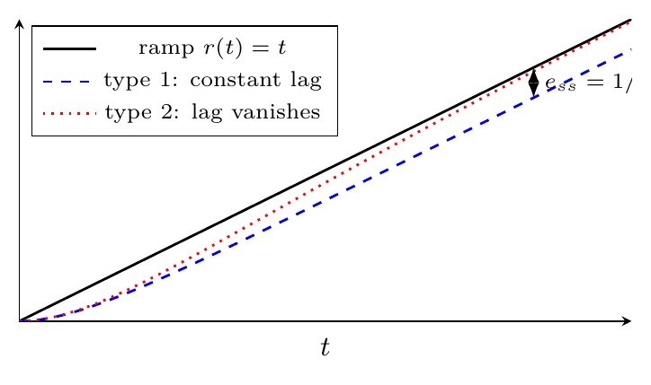
Ramp, $R = 1/s^2$. Now $e_{ss} = \lim 1/(s + sG(s)) = 1/\lim_{s\to0} sG(s)$. For type 0, $sG \to 0$ and the error grows without bound. For type 1, $sG(s) \to b_0/a_0$, a finite error $a_0/b_0$. For type 2, $sG\to\infty$ and $e_{ss} = 0$: the output eventually tracks the ramp exactly.
Parabola, $R = 1/s^3$. Here $e_{ss} = 1/\lim_{s\to0} s^2G(s)$, which is finite ($a_0/b_0$) only for type 2; types 0 and 1 give an unbounded error.
The nine results fit in one table:
| $e_{ss}$ | Step | Ramp | Parabola |
|---|---|---|---|
| Type 0 | $\dfrac{1}{1+G(0)}$ | $\infty$ | $\infty$ |
| Type 1 | $0$ | $\dfrac{a_0}{b_0}$ | $\infty$ |
| Type 2 | $0$ | $0$ | $\dfrac{a_0}{b_0}$ |
Many textbooks express the same results through the error constants $K_p = \lim G$, $K_v = \lim sG$ and $K_a = \lim s^2G$ (limits as $s\to0$), so that the three columns read $1/(1+K_p)$, $1/K_v$ and $1/K_a$.
The table shows a clear trend. More aggressive references are harder to track, and each integrator in the loop buys one more level of reference that can be tracked with zero error. For a ramp, the difference between type 1 and type 2 looks like this:
A design example
These results immediately support design. Suppose a type-0 plant has DC gain $G(0) = 10K/(14\cdot18)$, where $K$ is ours to choose, and we require the steady-state error to a unit step to be at most $10\%$. For type 0 and a step,
$$e_{ss} = \frac{1}{1 + G(0)} = \frac{14\cdot18}{14\cdot18 + 10K} = \frac{252}{252 + 10K} \le 0.1 \;\Longrightarrow\; 10K \ge 9\cdot252 = 2268 \;\Longrightarrow\; K \ge 226.8.$$As always, we must then confirm that the closed loop is stable at this gain.
Summary and outlook
- $E = S\,R$ with $S = 1/(1+G)$, and $T = 1 - S$ is the closed-loop transfer function.
- Check stability first, then apply the final value theorem.
- The type of the loop decides whether each reference is tracked with zero, finite or unbounded error.
We now have two families of specifications: transient ones (overshoot, settling and peak time, Lecture 7) and steady-state ones (this lecture). To meet them systematically, we need a design tool that shows how the closed-loop poles move as we change the controller. That tool is the root locus, introduced in the next lecture.
References
- N. S. Nise, Control Systems Engineering, 6th ed.: §7.1 Introduction (p. 340); §7.2 Steady-State Error for Unity Feedback Systems (p. 343); §7.3 Static Error Constants and System Type (p. 349); §7.4 Steady-State Error Specifications (p. 353); §7.7 Sensitivity (p. 362).
- X. Chen and M. Tomizuka, Introduction to Modern Controls, with Illustrations in MATLAB and Python: §3.1.2 Relevant Properties of the Laplace Transform (p. 36), for the final value theorem.