Lecture 26: Nyquist Stability: Worked Example, Gain and Phase Margins

Scheduled release: week of November 16, 2026.

Download lecture notes (PDF)

Introduction

A Nyquist sketch must contain enough geometric information to determine the signed encirclements of $-1$. Endpoints alone are often insufficient, especially when the loop has unstable poles. We construct a second-order example by calculating its axis crossings, then use the curve to find the stabilizing range of positive gain. This example leads naturally to gain and phase margins and to the effect of simultaneous gain and phase uncertainty. Negative unity feedback and counterclockwise-positive image winding are used throughout.

A loop with two unstable poles

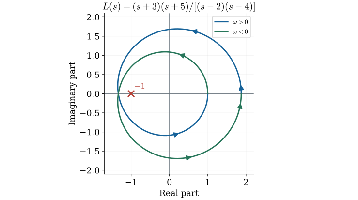
Consider a loop with poles at $2$ and $4$ and zeros at $-3$ and $-5$. The two unstable poles require two net counterclockwise encirclements of $-1$ for closed-loop stability. We first draw the response at unit gain, then use radial scaling to study other positive gains.

$$ L_K(s)=K\frac{(s+3)(s+5)}{(s-2)(s-4)},\qquad L_1(0)=\frac{15}{8},\quad L_1(\infty)=1. $$

The poles at $2$ and $4$ give $P=2$. No imaginary-axis indentation is needed. This loop is proper but not strictly proper, so its large-radius arc approaches $K$, not zero. Begin with $K=1$. To draw the curve faithfully, find the imaginary- and real-axis crossings, place them in frequency order, and then add the conjugate branch.

Substitute s equal to j omega

The low- and high-frequency values locate the ends of the positive-frequency branch, but the path between them remains unknown. Substituting $s=j\omega$ and expanding the polynomial factors is the first step toward finding its axis crossings.

$$ \begin{aligned}(j\omega+3)(j\omega+5)&=15-\omega^2+8j\omega,\\(j\omega-2)(j\omega-4)&=8-\omega^2-6j\omega,\\L_1(j\omega)&=\frac{15-\omega^2+8j\omega}{8-\omega^2-6j\omega}.\end{aligned} $$

The DC value and high-frequency limit locate the endpoints, but they do not determine the intermediate path. Expand the products, using $(j\omega)^2=-\omega^2$, so that the real and imaginary parts of each polynomial are visible. The next operation is division by a complex number. Multiply numerator and denominator by $8-\omega^2+6j\omega$ to make the denominator real.

Separate real and imaginary parts

To locate those crossings, write the complex quotient in terms of its real and imaginary parts. Multiplication by the conjugate denominator gives both parts a common real denominator. Its positivity allows the crossing conditions to be read from the numerator alone.

$$ L_1(j\omega)=\frac{\omega^4-71\omega^2+120+j\,14\omega(11-\omega^2)}{(8-\omega^2)^2+36\omega^2}. $$

The common denominator is strictly positive for real $\omega$. Thus an imaginary-axis crossing requires the real numerator to vanish; a real-axis crossing requires the imaginary numerator to vanish. These are different conditions. Preserve the $j^2=-1$ sign in the cross term: $(8j\omega)(6j\omega)=-48\omega^2$.

Collect the conjugate-product terms

The conjugate-product calculation is worth carrying out explicitly because its signs control the sketch. Products of two imaginary terms contribute to the real part with a negative sign; the cross terms supply the imaginary part. Collecting them gives two real polynomials in frequency.

$$ \begin{aligned}D_\omega&=(8-\omega^2)^2+36\omega^2,\\A_\omega&=(15-\omega^2)(8-\omega^2)-48\omega^2,\\B_\omega&=6\omega(15-\omega^2)+8\omega(8-\omega^2),\\L_1(j\omega)&=(A_\omega+jB_\omega)/D_\omega.\end{aligned} $$

The product of the two imaginary terms is $(8j\omega)(6j\omega)=-48\omega^2$ and belongs in the real numerator. The two cross terms belong in the imaginary numerator. Expanding gives $A_\omega=\omega^4-71\omega^2+120$ and $B_\omega=154\omega-14\omega^3$. Since $D_\omega$ is positive on the real frequency axis, axis crossings can be found directly from these numerator polynomials.

Imaginary-axis crossings

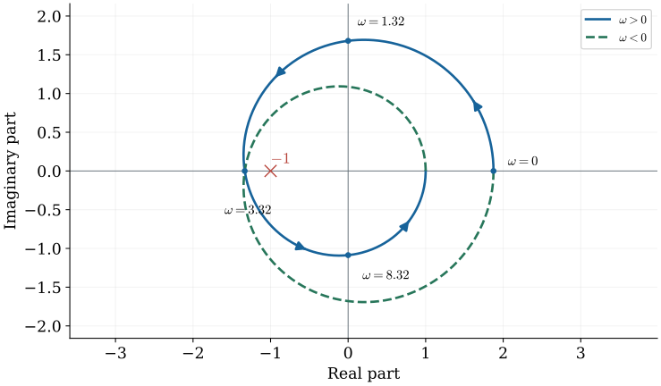
An imaginary-axis crossing occurs when the real part of the loop response vanishes. Its numerator is an even polynomial, so introducing $x=\omega^2$ reduces the crossing condition to a quadratic. Positive roots in $x$ give the positive crossing frequencies.

$$ x^2-71x+120=0,\qquad x=\frac{71\pm\sqrt{4561}}{2}. $$

The two positive frequencies are approximately $1.3162$ and $8.3227$ rad/s. The corresponding values of $L_1$ are approximately $+j1.6800$ and $-j1.0867$. The negative frequencies yield conjugate values. These checks anchor the curve and rule out a simple direct path from the initial point to the final point.

Place crossings in frequency order

The crossing frequencies determine when the curve meets the imaginary axis, but not the crossing heights. Substituting them into the imaginary part gives those coordinates. Placing the resulting points in increasing frequency order constrains the intermediate path and its orientation.

$$ \begin{array}{c|c}\omega&L_1(j\omega)\\\hline0&15/8\\1.3162&j1.6800\\8.3227&-j1.0867\\\infty&1\end{array} $$

The smaller positive root of the quadratic is reached first. Substitute each crossing frequency into $B_\omega/D_\omega$ to find its height on the imaginary axis. Join the points in increasing frequency order, with arrows. The connection between the two imaginary-axis crossings must cross the real axis; its location is still unknown. It matters because it determines whether the connection passes to the left or the right of $-1$.

The negative-real crossing and encirclements

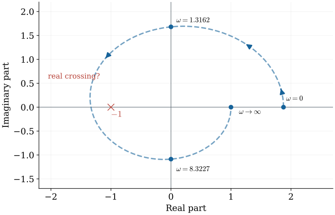
Between the two imaginary-axis crossings, the positive-frequency curve must cross the real axis. The position of this crossing relative to $-1$ is decisive for the winding count. For unit gain it lies to the left of the critical point, producing the encirclements needed to stabilize the two unstable poles.

$$ 14\omega(11-\omega^2)=0,\qquad \omega_{\mathrm{pc}}=\sqrt{11},\qquad L_1(j\sqrt{11})=-\frac{4}{3}. $$

The finite nonzero crossing is left of $-1$. The complete curve winds twice counterclockwise about $-1$, giving $N_{\mathrm{CCW}}=2$. With $P=2$, Nyquist gives $Z=0$. Direct verification at $K=1$ yields the characteristic polynomial $2s^2+2s+23$, whose roots are $-0.5\pm j\sqrt{45}/2$. Both have negative real part.

Solve the real-axis crossing condition

The crossing location follows by setting the imaginary numerator to zero. Besides the known zero-frequency point, the equation gives a nonzero positive frequency. Substitution into the real part provides the negative-real coordinate used in the preceding stability conclusion.

$$ \begin{aligned}B_\omega&=2\omega[3(15-\omega^2)+4(8-\omega^2)]\\&=14\omega(11-\omega^2),\\\omega&=0,\ \pm\sqrt{11},\\L_1(j\sqrt{11})&=\frac{121-781+120}{9+396}=-\frac43.\end{aligned} $$

The zero-frequency root is the known starting point. The nonzero roots give the additional real-axis crossing. Since $1.3162\lt \sqrt{11}\lt 8.3227$, the crossing occurs between the two imaginary-axis crossings, as required by the sketch. It is left of $-1$. Reflect the positive-frequency path, reverse its frequency order, and count two counterclockwise encirclements of the critical point.

Gain scaling and the exact stability interval

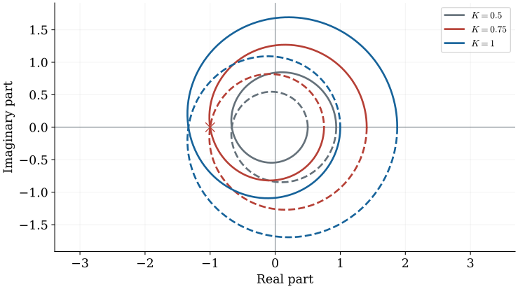
Once the unit-gain curve is known, changing a positive scalar gain requires no new frequency calculation. Every image point moves radially by the same factor. The stability boundary occurs when the negative-real crossing reaches $-1$, and the characteristic polynomial provides an independent check of the resulting gain interval.

$$ (1+K)s^2+(8K-6)s+(8+15K)=0,\qquad K\gt 0:\quad \text{stable iff }K\gt \frac34. $$

The boundary occurs when $-4K/3=-1$, so $K_{\mathrm{crit}}=0.75$. At the boundary the roots are $\pm j\sqrt{11}$, so the system is not asymptotically stable. For $0\lt K\lt 0.75$, there are two RHP roots; for $K\gt 0.75$, there are none. Relative to nominal $K=1$, the downward gain factor is $0.75$, or $20\log_{10}(0.75)\approx-2.499$ dB. There is no finite upper positive-gain stability boundary for this ideal model.

The critical gain reaches minus one

The geometric effect of the critical gain is now explicit. At the boundary, the frequency response passes through $-1$ and the closed loop has imaginary-axis characteristic roots. Further contraction and expansion place the curve on opposite sides of this boundary, so their effects on stability are different.

$$ \begin{aligned}L_K(j\sqrt{11})&=-4K/3,\\-4K/3=-1&\ \Longrightarrow\ K_{\mathrm{crit}}=3/4,\\0\lt K\lt 3/4:&\quad N_{\mathrm{CCW}}=0,\ Z=2,\\K\gt 3/4:&\quad N_{\mathrm{CCW}}=2,\ Z=0.\end{aligned} $$

Multiplication by a positive gain scales every coordinate by the same amount without changing phase or crossing frequency. At $K=3/4$, the curve touches $-1$ and the characteristic roots are $\pm j\sqrt{11}$. Further shrinking removes the two encirclements. Enlarging preserves them. This example therefore has a lower gain boundary; an increase in positive gain has no finite stability boundary in this ideal model.

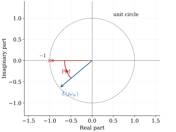
Phase margin as an angular clearance

Gain scaling changes distance from the origin. A phase perturbation instead changes angle, which motivates measuring angular clearance at a point where the loop magnitude is one. Such a point lies on the unit circle and can reach $-1$ through a change of phase alone.

$$ |L(j\omega_{\mathrm{gc}})|=1,\qquad \mathrm{PM}=180^\circ+\angle L(j\omega_{\mathrm{gc}}). $$

This is the usual additional-phase-lag convention for an appropriate stable nominal SISO loop and a selected gain crossover. Evaluate the continuous phase branch consistently. Multiple crossovers or unstable open-loop poles require the full Nyquist stability assessment; a single positive margin is not a universal stability proof. A physical real-coefficient perturbation also preserves conjugate symmetry; the rotation illustrates the positive-frequency geometry.

Read margins from Bode plots

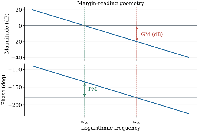
The same conditions can be read from Bode plots because they display the magnitude and phase of the same complex response. A magnitude of one corresponds to 0 dB, and the negative real axis corresponds to an odd multiple of $180^\circ$. Matching the appropriate crossings gives the conventional margin constructions.

$$ \mathrm{GM}=\frac{1}{|L(j\omega_{\mathrm{pc}})|},\qquad \mathrm{GM}_{\mathrm{dB}}=-20\log_{10}|L(j\omega_{\mathrm{pc}})|. $$

At a phase crossover the phase is an odd multiple of $180^\circ$; read the gain change needed to reach 0 dB. At a gain crossover, read the angular distance from the relevant $-180^\circ$ branch. Retain the direction of the gain change: a lower gain boundary such as $0.75$ must not be misreported as tolerance to an increase.

Joint gain and phase uncertainty

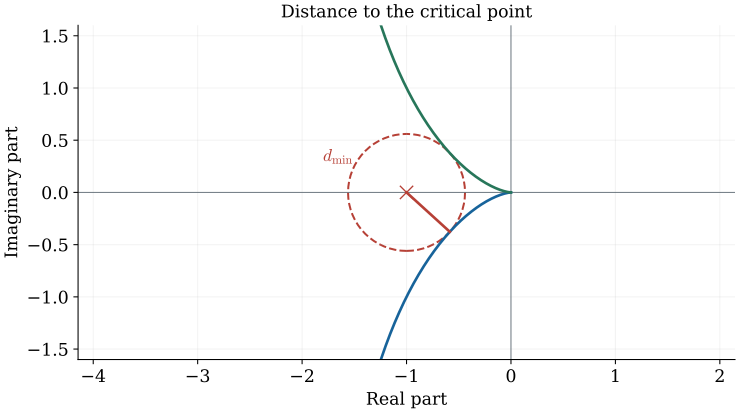
Separate gain and phase margins consider one type of change at a time. Real uncertainty can change both together, so a broader geometric view asks how close the loop curve comes to $-1$. This distance also connects the Nyquist picture to the sensitivity function $S(s)=1/(1+L(s))$.

$$ d_{\min}=\min_\omega|1+L(j\omega)|,\qquad S(s)=\frac{1}{1+L(s)}. $$

The distance from a point on the loop curve to $-1$ is $|1+L(j\omega)|$. Its minimum is the modulus margin, which is related to the peak sensitivity by $d_{\min}=1/\|S\|_\infty$ when the frequency supremum is appropriate. A formal disk margin describes an admissible family of simultaneous multiplicative gain and phase perturbations; it is not in general the same as the shortest Euclidean distance. The geometric motivation is to prevent the perturbed loop curve from reaching the critical point.

Perspective

Axis crossings and traversal directions turn an approximate Nyquist drawing into a stability calculation. In the worked example, the stabilizing condition is $K\gt 3/4$ for positive gain, illustrating that reducing gain can destabilize a loop with unstable poles. Gain and phase margins describe selected ways of reaching the critical point, while the sensitivity relation helps interpret joint changes. All of these measures must be read in the context of the complete Nyquist count.

This completes the technical frequency-domain sequence.

References

Norman S. Nise, Control Systems Engineering, 6th ed., Wiley, 2011.

• §§10.4–10.7: Nyquist construction, stability, and margins.
• §6.2: Routh-Hurwitz stability check.
• §7.7: Sensitivity.