Lecture 15: High-Order Poles and the Root Locus
Lecture 8 established that a pole far to the left of the dominant poles barely affects the transient response, so it can often be ignored. This lecture adds a warning. The same fast pole can change the closed-loop design freedom a great deal, and the root locus shows this at a glance.
A motion-control example
The block diagram below shows a typical motion-control loop: a gain $K$, a power amplifier and a motor.
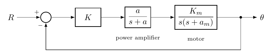
The motor model follows from Newton’s law, $F = ma$. A voltage or force produces acceleration, and integrating twice gives position. In practice, friction and damping make one of the integrations imperfect, which gives $\dfrac{K_m}{s(s+a_m)}$ with a small $a_m$ (here $a_m = 1.71$). The power amplifier boosts the small control signal to the voltage or current the motor needs. It is modelled as $\dfrac{a}{s+a}$ with a fast pole, $a = 100$. The only design freedom is the gain $K$.
The open-loop poles are therefore $0$, $-1.71$ and $-100$. By the reasoning of Lecture 8, the pair at $0$ and $-1.71$ is dominant, and the pole at $-100$, more than fifty times further left, contributes a transient that decays almost instantly. It is tempting to drop it. The root locus shows what that would cost.
Root locus with and without the fast pole
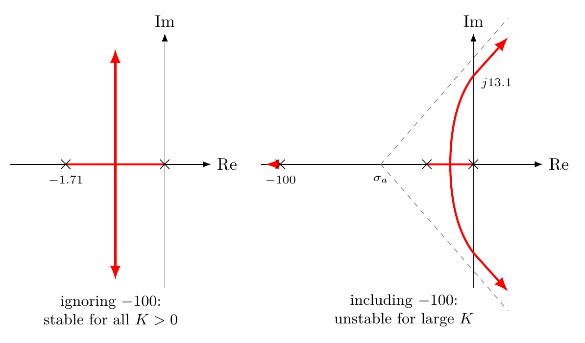
Without the fast pole, there are two poles and no zeros ($n - m = 2$), so the asymptotes are at $\pm90^\circ$. The branches meet at $-0.855$ and go straight up and down, always in the left half-plane. The loop appears stable for any gain.
With the fast pole, $n - m = 3$, and the asymptotes are at $\pm60^\circ$ and $180^\circ$, with centroid
$$\sigma_a = \frac{0 - 1.71 - 100}{3} = -\frac{101.71}{3} \approx -33.9.$$The dominant branches now bend toward the $\pm60^\circ$ asymptotes and cross into the right half-plane at high gain.
The Routh array locates the crossing exactly. With total loop gain $K' = K\,a\,K_m$, the characteristic polynomial is $s^3 + 101.71\,s^2 + 171\,s + K'$. The loop is stable for $K' \lt 101.71\times171 \approx 1.74\times10^4$, and the branches cross the imaginary axis at $s = \pm j\sqrt{171} \approx \pm j13.1$.
The fast pole leaves the transient almost untouched, but it changes the asymptotes, and with them the maximum gain the loop can tolerate.
Summary and outlook
- A non-dominant pole has little effect on the transient, but it changes the asymptotes and therefore the stability limits of the closed loop.
- Keep fast poles in the model when judging how much gain a loop can tolerate.
- The root locus gives this insight without computing any roots, which is why analytical tools still matter alongside computation.
Root-locus design places closed-loop poles, so it pays to have a sharp intuition for how each pole location translates into a time response. The next lecture develops that intuition.
References
- N. S. Nise, Control Systems Engineering, 6th ed.: §4.7 System Response with Additional Poles (p. 186); §8.4 Sketching the Root Locus (p. 397); §8.7 Transient Response Design via Gain Adjustment (p. 415).