Lecture 4: The Laplace Transform
Lecture 3 showed that physical systems are modeled by ordinary differential equations. Solving an ODE directly, in the time domain, can be tedious: we guess a solution form, differentiate, match coefficients and fit initial conditions. This lecture reviews the tool that replaces all of that with algebra, the Laplace transform. We define it, check when it exists, compute the transforms we will use throughout the course, take a careful look at the Dirac impulse, and collect the properties that make the transform so useful.
A warm-up puzzle
What is the value of
$$\sum_{n=1}^{\infty}\frac{(-1)^{n+1}}{n} = 1 - \frac12 + \frac13 - \frac14 + \cdots\ ?$$It is not obvious how to sum this series, and it is even less obvious what it has to do with differential equations. Keep it in mind; we will answer it with the Laplace transform once the first few examples are in place.
The Laplace approach to ODEs
The transform is named after Pierre-Simon Laplace (1749–1827), sometimes called “the French Newton.” He was 13 years younger than Lagrange and studied under Jean le Rond d’Alembert, who co-discovered the fundamental theorem of algebra (also known as the d’Alembert/Gauss theorem).
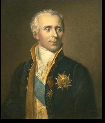
Pierre-Simon Laplace (1749–1827).
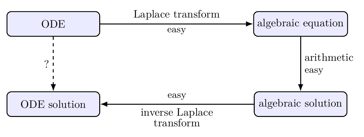
The idea behind the Laplace approach is a detour that turns out to be shorter than the direct road. Going straight from an ODE to its solution is hard. Instead, we transform the ODE into an algebraic equation, which is easy; solve the algebra with arithmetic, which is easy; and transform the algebraic solution back to the time domain with the inverse Laplace transform, which is also easy once we have a table of transform pairs (Lecture 5).
Definition
We work with continuous-time functions $f:\mathbb{R}_+\to\mathbb{R}$. The domain of $f$ is the nonnegative real numbers and its values are real. We write $f(t)$ and assume throughout that $f(t) = 0$ for all $t\lt 0$. (Notation: $\mathbb{R}$ and $\mathbb{C}$ are the real and complex numbers, $\in$ means “belongs to,” and $\triangleq$ means “defined as.”)
The Laplace transform of $f(t)$ is
$$F(s) = \mathcal{L}\{f(t)\} \triangleq \int_0^\infty f(t)\,e^{-st}\,dt, \qquad s\in\mathbb{C}.$$The transform takes a function of time and returns a function of the complex variable $s$.
Existence
The integral does not converge for every function. Two conditions together are sufficient:
- $f(t)$ is piecewise continuous: it may jump, but only finitely many times on any finite interval.
- $f(t)$ does not grow faster than an exponential as $t\to\infty$: there are constants $k,\alpha,t_0\in\mathbb{R}_+$ such that $|f(t)| \lt k e^{\alpha t}$ for all $t\ge t_0$.
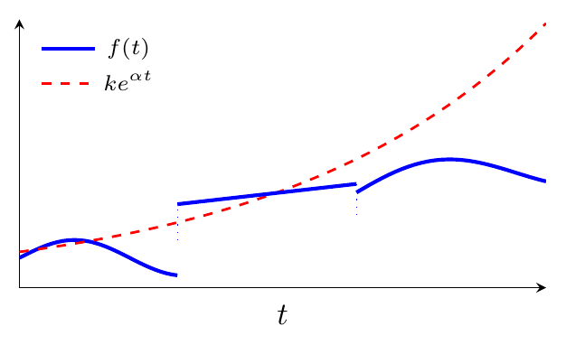
Under the second condition, $e^{-st}$ wins against $f(t)$ whenever $\mathrm{Re}\,s \gt \alpha$, so the integral converges there. All the signals in this course, including growing exponentials from unstable systems, satisfy both conditions. A function such as $e^{t^2}$ does not.
Basic examples
Exponential. For $f(t) = e^{-at}$, $a\in\mathbb{C}$,
$$F(s) = \int_0^\infty e^{-at}e^{-st}\,dt = \left[\frac{-e^{-(s+a)t}}{s+a}\right]_0^\infty = \frac{1}{s+a} \qquad (\mathrm{Re}\,s \gt -\mathrm{Re}\,a).$$Unit step. Setting $a=0$ gives the transform of the unit step $1(t) = 1$ for $t\ge0$ (and $0$ for $t\lt 0$):
$$\mathcal{L}\{1(t)\} = \frac{1}{s}.$$Back to the puzzle. The step transform says that, for any positive integer $n$,
$$\frac{1}{n} = \int_0^\infty e^{-nt}\,dt,$$since this is $\mathcal{L}\{1(t)\}$ evaluated at $s=n$. Substituting into the series and exchanging the sum and the integral,
$$\sum_{n=1}^{\infty}\frac{(-1)^{n+1}}{n} = \int_0^\infty\sum_{n=1}^{\infty}(-1)^{n+1}e^{-nt}\,dt = \int_0^\infty\frac{e^{-t}}{1+e^{-t}}\,dt = \Big[-\ln\left(1+e^{-t}\right)\Big]_0^\infty = \ln 2 .$$The inner sum is a geometric series with ratio $-e^{-t}$. The Laplace integral turned an awkward infinite sum into a geometric series and one elementary integral.
Sine and cosine. Euler’s formula $e^{ja} = \cos a + j\sin a$ gives
$$\sin(\omega t) = \frac{e^{j\omega t}-e^{-j\omega t}}{2j}, \qquad \cos(\omega t) = \frac{e^{j\omega t}+e^{-j\omega t}}{2}.$$With $\mathcal{L}\{e^{j\omega t}\} = 1/(s-j\omega)$ from the exponential example,
$$\mathcal{L}\{\sin\omega t\} = \frac{1}{2j}\left(\frac{1}{s-j\omega}-\frac{1}{s+j\omega}\right) = \frac{\omega}{s^2+\omega^2}, \qquad \mathcal{L}\{\cos\omega t\} = \frac{s}{s^2+\omega^2}.$$Leonhard Euler (1707–1783), a student of Johann Bernoulli and teacher of Lagrange, wrote 380 articles in 25 years at Berlin and was still producing about one paper per week at age 67, when he was almost blind.
The Dirac impulse
The Dirac impulse $\delta(t-T)$ is an infinitely tall, infinitely narrow pulse at $t=T$ with unit area. It is not an ordinary function but a generalized function (formally, a distribution). Why do we need it? Consider
$$\dot y - ay = \dot u + bu .$$If $u$ is the unit step $1(t)$, then $u$ jumps at $t=0$ and $\dot u$ cannot be evaluated there in the ordinary sense. We need a meaning for “the derivative of a jump.”
First-order approximation. Replace the step by a ramp that rises from 0 to 1 over a short time $\epsilon$:
$$\mu_\epsilon(t) = \begin{cases}0 & t\lt 0\\ t/\epsilon & 0\le t\lt \epsilon\\ 1 & \epsilon\le t\end{cases} \qquad\Longrightarrow\qquad \dot\mu_\epsilon(t) = \begin{cases}0 & t\lt 0\\ 1/\epsilon & 0\lt t\lt \epsilon\\ 0 & \epsilon\lt t .\end{cases}$$As $\epsilon\to0$, $\mu_\epsilon$ approaches the unit step, and its derivative becomes a taller and narrower rectangle whose area stays equal to 1.
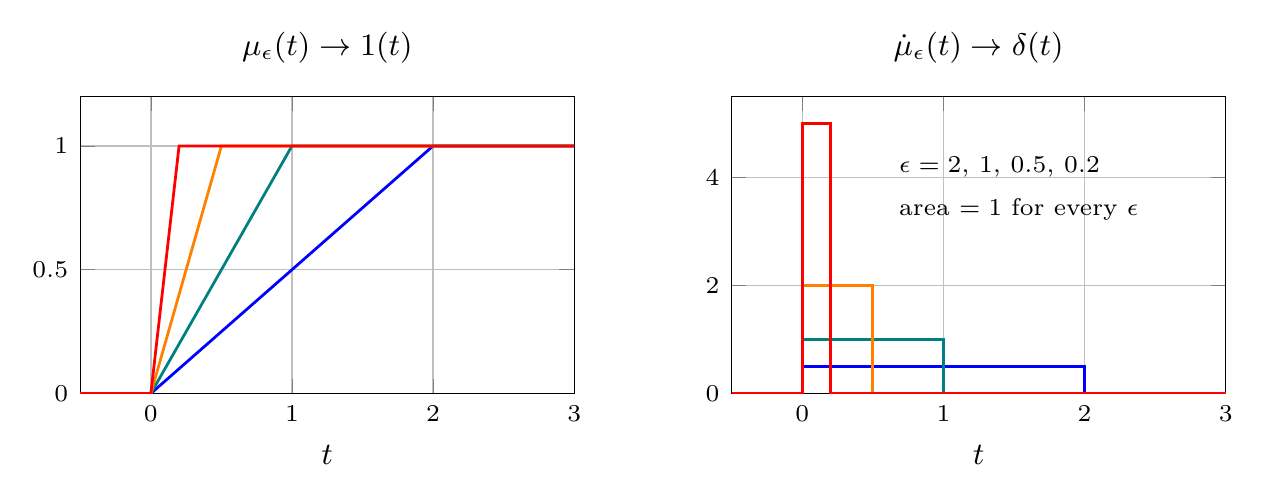
Two properties of the rectangle survive the limit:
$$\int_{-\infty}^{\infty}\dot\mu_\epsilon(t)\,dt = 1, \qquad \lim_{\epsilon\to0}\int_{-\infty}^{\infty} f(t)\,\dot\mu_\epsilon(t)\,dt = \lim_{\epsilon\to0}\int_0^\epsilon f(t)\frac1\epsilon\,dt = f(0)$$for any $f$ continuous at 0. They define the impulse:
$$\int_0^\infty \delta(t-T)\,dt = 1, \qquad \int_0^\infty \delta(t-T)f(t)\,dt = f(T) .$$The second is the sifting property: integrating against $\delta(t-T)$ picks out the value of $f$ at $T$.
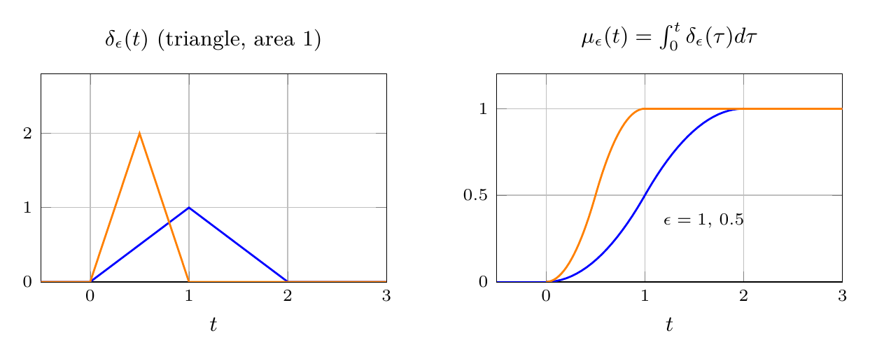
Smoother approximations. The ramp approximation $\mu_\epsilon$ is only once differentiable, and its derivative $\dot\mu_\epsilon$ is itself discontinuous. It cannot handle an equation with $\ddot u$, such as $\ddot y + 2\dot y - ay = \ddot u + 3\dot u + bu$. A triangular pulse fixes this:
$$\delta_\epsilon(t) = \begin{cases} 0 & t\lt 0\\ t/\epsilon^2 & 0\lt t\lt \epsilon\\ (2\epsilon-t)/\epsilon^2 & \epsilon\lt t\lt 2\epsilon\\ 0 & 2\epsilon\lt t\end{cases}$$has unit area, and its integral $\mu_\epsilon(t) = \int_0^t\delta_\epsilon(\tau)\,d\tau$ is a smoother approximation of the unit step that is twice differentiable. The process can be repeated to make $\delta_\epsilon$ as smooth as we like, even infinitely differentiable.
An application. The same idea, tracking how a nonsmooth signal propagates through smoother and smoother approximations, is used in research on add-on servo control, where a plug-in controller that switches on can inject a nonsmooth signal into a precision system. See T. Jiang and X. Chen, “Transmission of signal nonsmoothness and transient improvement in add-on servo control,” IEEE Transactions on Control Systems Technology.
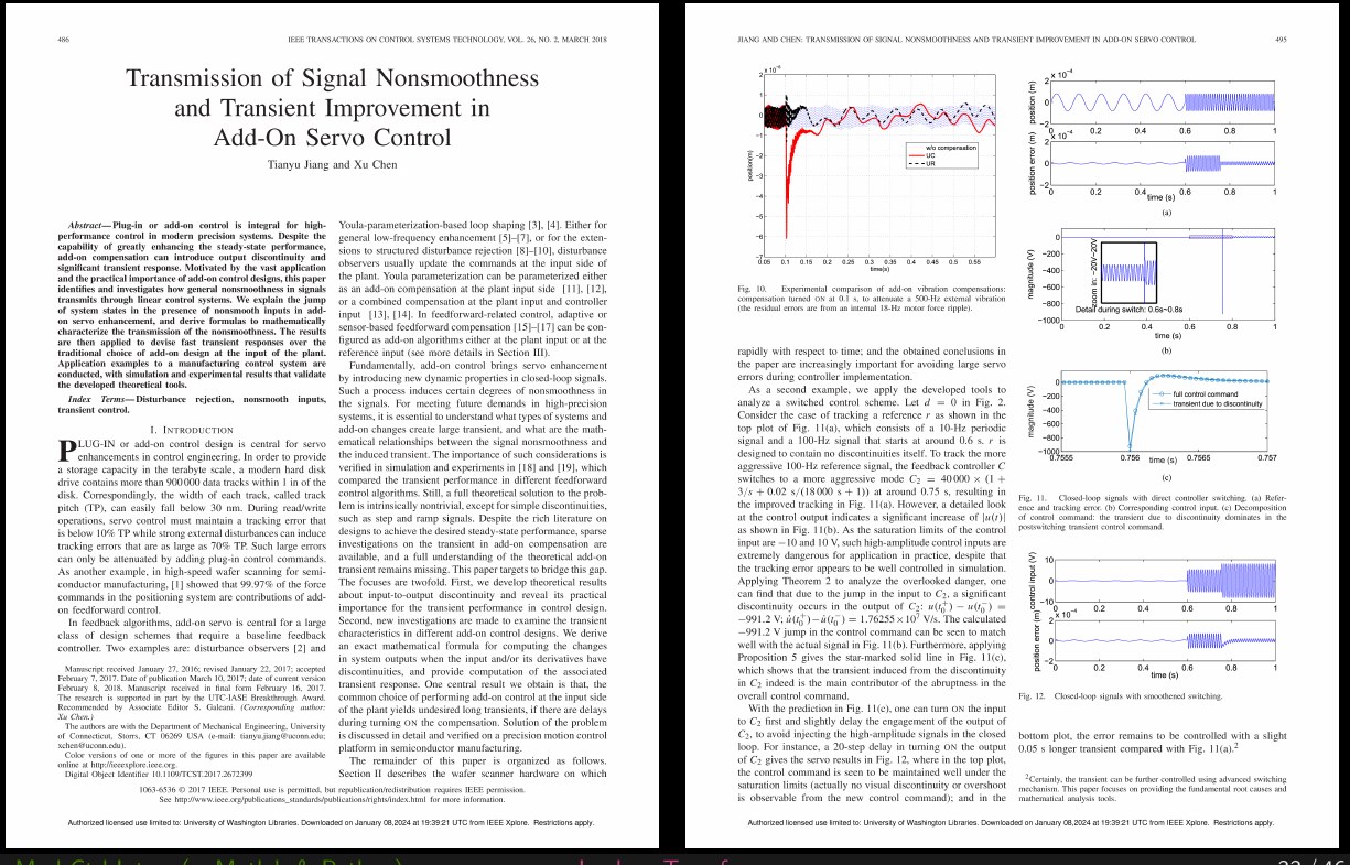
Jiang and Chen, “Transmission of signal nonsmoothness and transient improvement in add-on servo control.”
Transform of the impulse. By the sifting property,
$$\mathcal{L}\{\delta(t)\} = \int_0^\infty e^{-st}\delta(t)\,dt = e^{-s\cdot0} = 1 .$$The impulse is the one signal whose transform is the constant 1. We will see shortly why this makes it so important.
Properties of the Laplace transform
Throughout, let $F(s) = \mathcal{L}\{f(t)\}$ and $G(s) = \mathcal{L}\{g(t)\}$.
Linearity. For any $\alpha,\beta\in\mathbb{C}$,
$$\mathcal{L}\{\alpha f(t) + \beta g(t)\} = \alpha F(s) + \beta G(s).$$This follows directly from the linearity of the integral. We already used it for the sine and cosine.
Differentiation.
$$\mathcal{L}\{\dot f(t)\} = sF(s) - f(0).$$Integration by parts gives
$$\mathcal{L}\{\dot f(t)\} = \int_0^\infty e^{-st}\dot f(t)\,dt = -\int_0^\infty\frac{de^{-st}}{dt}f(t)\,dt + \Big[e^{-st}f(t)\Big]_{t=0}^{t\to\infty} = s\int_0^\infty e^{-st}f(t)\,dt - f(0) = sF(s) - f(0).$$This is the property that turns differential equations into algebra: differentiation in time becomes multiplication by $s$, with the initial condition appearing as an extra term. Applying it twice, $\mathcal{L}\{\ddot f\} = s^2F(s) - sf(0) - \dot f(0)$.
Integration. Integration is the inverse of differentiation, and correspondingly
$$\mathcal{L}\left\{\int_0^t f(\tau)\,d\tau\right\} = \frac{1}{s}F(s).$$Multiplication by $e^{-at}$ (frequency shift).
$$\mathcal{L}\{e^{-at}f(t)\} = F(s+a).$$For example, from $\mathcal{L}\{1(t)\} = 1/s$ we recover $\mathcal{L}\{e^{-at}\} = 1/(s+a)$, and from $\mathcal{L}\{\sin\omega t\} = \omega/(s^2+\omega^2)$ we obtain the damped sine
$$\mathcal{L}\{e^{-at}\sin\omega t\} = \frac{\omega}{(s+a)^2+\omega^2}.$$This pair will describe every underdamped response in the course.
Multiplication by $t$.
$$\mathcal{L}\{t f(t)\} = -\frac{dF(s)}{ds}.$$For example, $\mathcal{L}\{1(t)\} = 1/s$ gives $\mathcal{L}\{t\} = 1/s^2$, and repeating gives $\mathcal{L}\{t^2\} = 2/s^3$ and $\mathcal{L}\{te^{-at}\} = 1/(s+a)^2$.
Time delay. A signal delayed by $\tau$ picks up an exponential factor:
$$\mathcal{L}\{f(t-\tau)\} = e^{-s\tau}F(s).$$In particular, $\mathcal{L}\{\delta(t-T)\} = e^{-sT}$.
Convolution. Define the convolution
$$(f\star g)(t) = \int_0^t f(t-\tau)g(\tau)\,d\tau = (g\star f)(t).$$Then
$$\mathcal{L}\{(f\star g)(t)\} = F(s)G(s).$$This property explains the importance of the impulse. For an LTI system, the output is the convolution of the input with the system’s impulse response $g(t)$. In the Laplace domain the convolution becomes a product, $Y(s) = G(s)U(s)$. If the input is an impulse, $U(s)=1$, so $Y(s) = G(s)\times1$: the transfer function $G(s)$ is exactly the Laplace transform of the impulse response, $g(t) = \mathcal{L}^{-1}\{G(s)\}$.

Initial and final value theorems
Two theorems let us read off the beginning and end of a signal directly from its transform, without inverting it.
Initial value theorem. If $f(0^+) = \lim_{t\to0^+}f(t)$ exists, then
$$f(0^+) = \lim_{s\to\infty} sF(s).$$Final value theorem (FVT). If $\lim_{t\to\infty}f(t)$ exists, then
$$\lim_{t\to\infty} f(t) = \lim_{s\to0} sF(s).$$The condition matters. Consider two examples:
$$Y_1(s) = \frac{3(s+2)}{s(s^2+2s+10)}, \qquad Y_2(s) = \frac{3}{s-2}.$$For $Y_1$, the poles of $sY_1(s) = 3(s+2)/(s^2+2s+10)$ are $-1\pm3j$, in the left half-plane, so $y_1(t)$ settles and the FVT applies:
$$\lim_{t\to\infty}y_1(t) = \lim_{s\to0}\frac{3(s+2)}{s^2+2s+10} = \frac{6}{10} = 0.6 .$$For $Y_2$, blindly applying the formula gives $\lim_{s\to0}3s/(s-2) = 0$. But $y_2(t) = 3e^{2t}$ grows without bound, so $\lim_{t\to\infty}y_2(t)$ does not exist and the FVT does not apply. Before using the FVT, always check that all poles of $sF(s)$ are in the open left half-plane. Lecture 12 will use the FVT constantly to compute steady-state errors.
Common Laplace transform pairs
| $f(t)$ | $F(s)$ | $f(t)$ | $F(s)$ |
|---|---|---|---|
| $\delta(t)$ | $1$ | $e^{-at}$ | $\dfrac{1}{s+a}$ |
| $1(t)$ | $\dfrac1s$ | $t$ | $\dfrac{1}{s^2}$ |
| $\sin\omega t$ | $\dfrac{\omega}{s^2+\omega^2}$ | $t^2$ | $\dfrac{2}{s^3}$ |
| $\cos\omega t$ | $\dfrac{s}{s^2+\omega^2}$ | $te^{-at}$ | $\dfrac{1}{(s+a)^2}$ |
| $t\,x(t)$ | $-\dfrac{dX(s)}{ds}$ | $e^{-at}\sin\omega t$ | $\dfrac{\omega}{(s+a)^2+\omega^2}$ |
| $\dfrac{x(t)}{t}$ | $\displaystyle\int_s^\infty X(\sigma)\,d\sigma$ | $e^{-at}\cos\omega t$ | $\dfrac{s+a}{(s+a)^2+\omega^2}$ |
From ODEs to transfer functions
We can now carry out the first step of the Laplace approach. Take the mass-spring-damper of Lecture 3, $m\ddot y + b\dot y + ky = u$, and apply the differentiation property:
$$m\left[s^2Y(s) - sy(0) - \dot y(0)\right] + b\left[sY(s) - y(0)\right] + kY(s) = U(s).$$With zero initial conditions this is simply $(ms^2+bs+k)\,Y(s) = U(s)$, and
$$\frac{Y(s)}{U(s)} = \frac{1}{ms^2+bs+k} .$$The ODE has become a ratio of polynomials, the transfer function. In general, the $n$th-order ODE of Lecture 3 gives
$$G(s) = \frac{Y(s)}{U(s)} = \frac{b_ms^m + \cdots + b_1s + b_0}{s^n + a_{n-1}s^{n-1} + \cdots + a_0}.$$Summary and outlook
- The Laplace transform $F(s) = \int_0^\infty f(t)e^{-st}\,dt$ exists for piecewise-continuous functions of at most exponential growth.
- Key pairs: $\delta\to1$, $1(t)\to1/s$, $e^{-at}\to1/(s+a)$, $\sin\omega t\to\omega/(s^2+\omega^2)$, $\cos\omega t\to s/(s^2+\omega^2)$.
- The impulse is the limit of unit-area pulses; its sifting property gives $\mathcal{L}\{\delta\}=1$.
- Differentiation becomes multiplication by $s$; convolution becomes multiplication. So the transfer function is the transform of the impulse response.
- The FVT gives $\lim_{t\to\infty}f(t) = \lim_{s\to0}sF(s)$, but only when that limit exists.
We have completed the first two legs of the Laplace detour: ODE to algebra, and algebra to an algebraic solution. The next lecture completes the third leg, the return trip to the time domain through the inverse Laplace transform and partial fractions.
References
- N. S. Nise, Control Systems Engineering, 6th ed.: §2.2 Laplace Transform Review (p. 35), including Tables 2.1 and 2.2; §2.3 The Transfer Function (p. 44); §7.2 Steady-State Error for Unity Feedback Systems (p. 343), for the final value theorem in use.
- X. Chen and M. Tomizuka, Introduction to Modern Controls, with Illustrations in MATLAB and Python: §3.1 The Laplace Transform (p. 29); §3.1.1 The Laplace Approach to ODEs (p. 29); §3.1.2 Relevant Properties of the Laplace Transform (p. 36); §3.3 From Laplace Transform to Transfer Functions (p. 41).