Lecture 3: Modeling of Dynamic Systems
Lecture 1 ended with a five-step path: model the plant, analyze it, design a controller, analyze the closed loop, and implement. Lecture 2 then gave us the language of block diagrams for connecting models once we have them. This lecture goes back to the first step and asks where a model comes from, what forms it can take, and which properties of a model matter for control. We will also see why every model is an approximation, and why feedback lets us succeed anyway.
Why modeling?
Watch a slow-motion video of a thin beam that has been struck: it does not just move, it bends and rings in a characteristic shape, its third mode of vibration. If we want to suppress that ringing, we must first understand it. This is the general case: only when we have a good understanding of a system can we optimally control it. A model lets us
- simulate and predict the actual system response before building or testing hardware, and
- design model-based controllers, the approach taken throughout this course.
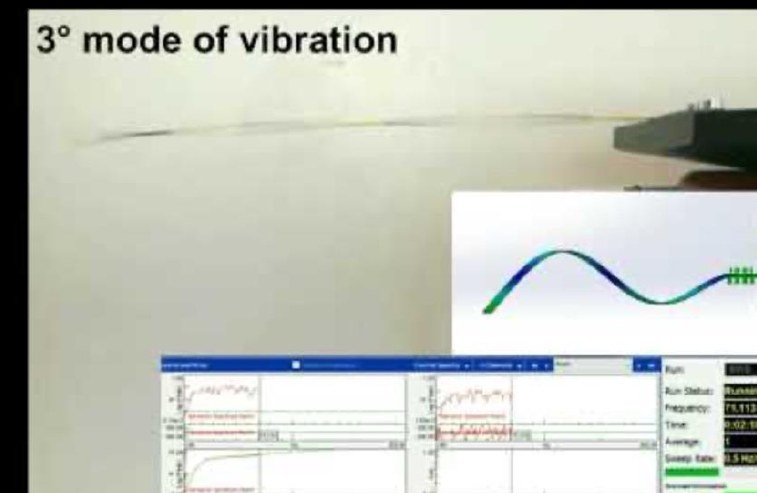
Why modeling: the third mode of vibration of a thin beam, captured in slow motion and compared with its predicted mode shape.
Two approaches to modeling
There are two broad ways to obtain a model:
- Based on physics. Apply fundamental engineering principles, such as Newton’s laws, energy conservation or Kirchhoff’s laws, to write equations that describe the system.
- Based on measurement data. Excite the system, record its input-output response, and fit a model to the data. This is a field of its own, known as system identification.
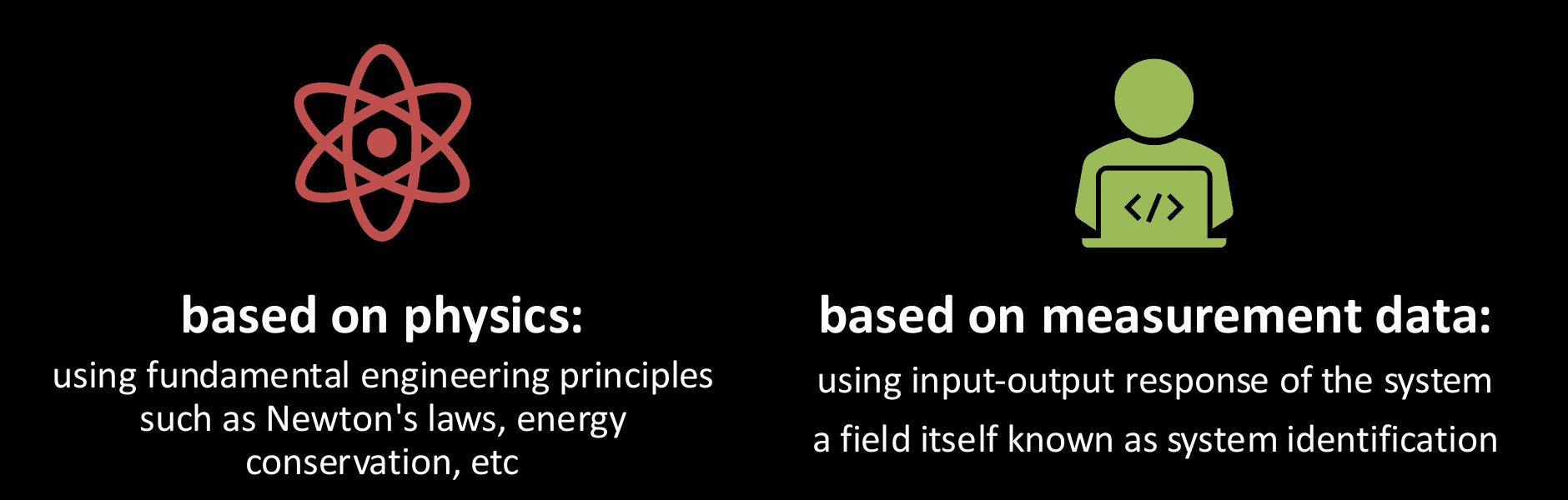
The two general approaches to modeling.
In practice the two are combined: physics suggests the structure of the model (its order, which terms appear), and data fixes the numbers. The hard-disk-drive example below shows exactly this.
Example: the mass-spring-damper
The simplest mechanical model, and one we will return to again and again, is a mass $m$ attached to a wall through a spring $k$ and a damper $b$, pushed by an external force $u = F$.
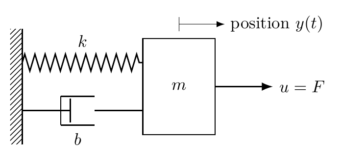
Newton’s second law, $F = ma$, applied to the mass gives
$$m\ddot y(t) + b\dot y(t) + k y(t) = u(t), \qquad y(0) = y_0,\quad \dot y(0) = \dot y_0 .$$The spring force $ky$ pulls the mass back toward its rest position, the damper force $b\dot y$ opposes the velocity, and whatever is left over accelerates the mass. The result is a second-order ordinary differential equation (ODE) with input $u(t)$ and output $y(t)$. Two initial conditions, position and velocity, are needed to fix the solution. Lecture 7 studies its step response in detail; for now, the point is that one physical law produced a complete dynamic model.
Example: hard-disk-drive actuator
Our second example returns to the hard-disk drive of Lecture 1. The read/write head sits at the tip of an actuator arm that rotates about a pivot, driven by a voice-coil motor (VCM).
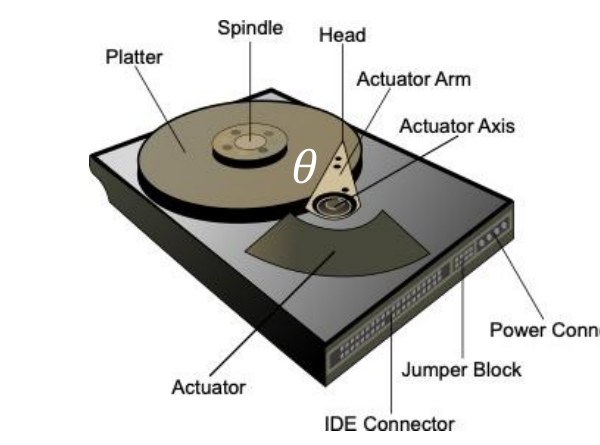
Main parts of a hard-disk drive: the actuator arm rotates by an angle $\theta$ about the actuator axis.
Rigid-body model. Newton’s second law for rotation says that the net torque equals the moment of inertia times the angular acceleration, $\tau = J\alpha$. Taking the arm angle $\theta$ as the output and the torque $\tau$ as the input,
$$\ddot\theta = \alpha = \frac{1}{J}\tau \quad\Longleftrightarrow\quad \theta(s) = \frac{1}{Js^2}T(s),$$where the right-hand form uses the Laplace transform, which Lectures 4 and 5 review. A double integrator: push with a constant torque and the angle grows quadratically.
Adding damping. The pivot bearing and air drag add damping, and the flex cable connecting the arm to the electronics adds a small stiffness:
$$\ddot\theta + 2\zeta\omega_n\dot\theta + \omega_n^2\theta = \kappa\tau \quad\Longleftrightarrow\quad \theta(s) = \frac{\kappa}{s^2+2\zeta\omega_n s+\omega_n^2}T(s).$$This has the same structure as the mass-spring-damper.
Adding the structural modes. The arm is not perfectly rigid. Like the vibrating beam, it bends and twists at many resonant frequencies. Each resonance $i$ behaves like its own lightly damped mass-spring-damper, $\ddot\theta_i + 2\zeta_i\omega_i\dot\theta_i + \omega_i^2\theta_i = \kappa_i\tau$, and the measured angle is the sum of all of them. The final model is
$$\theta(s) = \sum_{i=1}^{n} \frac{\kappa_i}{s^2+2\zeta_i\omega_i s+\omega_i^2}\,T(s),$$with the rigid-body mode as the term $i=1$ ($\omega_1 = 0$, $\zeta_1 = 0$).
Physics gave the structure of this model; the numbers $\kappa_i$, $\omega_i$, $\zeta_i$ come from measured frequency responses. The following Python code builds a 16-mode model with realistic values (a VCM gain of $3.7976\times10^7$ and resonances between 5.3 and 44.8 kHz).
import numpy as np
import control as ct

Kp_vcm = 3.7976e7                                  # VCM gain
omega_vcm = np.array([0, 5300, 6100, 6500, 8050, 9600, 14800, 17400, 21000,
                      26000, 26600, 29000, 32200, 38300, 43300, 44800]) * 2 * np.pi
kappa_vcm = np.array([1, -1.0, 0.1, -0.1, 0.04, -0.7, -0.2, -1.0, 3.0,
                      -3.2, 2.1, -1.5, 2.0, -0.2, 0.3, -0.5])
zeta_vcm = np.array([0, 0.02, 0.04, 0.02, 0.01, 0.03, 0.01, 0.02, 0.02,
                     0.012, 0.007, 0.01, 0.03, 0.01, 0.01, 0.01])

P = ct.tf([0], [1])                                # start from an empty transfer function
for k, w, z in zip(kappa_vcm, omega_vcm, zeta_vcm):
    P = P + ct.tf([k * Kp_vcm], [1, 2 * z * w, w**2])
The same model is a few lines of MATLAB with tf in a loop. Its frequency response, the Bode plot
we will study in the frequency-domain part of the course, is shown below. At low frequency the
gain falls at $-40$ dB per decade and the phase is $-180^\circ$, exactly the double integrator.
Above about 5 kHz the resonances appear as sharp peaks and phase jumps.
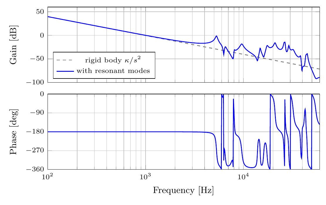
The rigid-body model is adequate for designing a controller that works well below the first resonance. A high-performance servo that pushes the bandwidth up must account for the resonances too. Choosing how much detail to keep is itself an engineering decision.
Models of continuous-time systems
Both examples are special cases of the general linear continuous-time model, an $n$th-order ODE relating the input $u$ to the output $y$:
$$\frac{d^n y}{dt^n} + a_{n-1}\frac{d^{n-1} y}{dt^{n-1}} + \cdots + a_0 y = b_m\frac{d^m u}{dt^m} + b_{m-1}\frac{d^{m-1} u}{dt^{m-1}} + \cdots + b_0 u,$$with initial conditions $y(0)=y_0,\ \dots,\ y^{(n-1)}(0)=y_0^{(n-1)}$. The mass-spring-damper has $n=2$, $m=0$. Lecture 4 will turn every such ODE into an algebraic equation in the Laplace variable $s$, and the ratio of the output to the input polynomial will be the transfer function.
Models of discrete-time systems
Many signals exist only at discrete instants $k = 1, 2, \dots$: sampled sensor readings, a digital controller’s output, or a monthly bank balance. They are described by difference equations:
$$y(k) + a_{n-1}y(k-1) + \cdots + a_0 y(k-n) = b_m u(k+m-n) + \cdots + b_0 u(k-n).$$Example: a bank account. Let $x(k)$ be the balance immediately before the deposit at the beginning of month $k$, $u(k)$ the deposit made at that instant, and $\rho$ the monthly interest rate. Deposit first, then credit one month’s interest:
$$x(k+1) = (1+\rho)\bigl(x(k)+u(k)\bigr), \qquad x(0) = x_0 .$$Deposit USD 100 at the beginning of each month for 30 years (360 deposits), starting from $x_0=0$. The nominal annual interest rate is 4%, compounded monthly, so $\rho=0.04/12$. After the 360th month, before any further deposit, the total deposited is USD 36,000 and the balance is
$$x(360)=100(1+\rho)\frac{(1+\rho)^{360}-1}{\rho} \approx \text{USD }69{,}636.29.$$To derive this, write $a=1+\rho$ and take a constant monthly deposit $u$. Then $x(1)=au$, $x(2)=a^2u+au$, and, with $x(0)=0$,
$$x(N)=u(a+a^2+\cdots+a^N)=ua\frac{a^N-1}{a-1}.$$The first deposit earns interest for 360 months and the last for one month. Interest earned is USD 33,636.29. The model assumes a fixed rate, no fees or withdrawals, and no rounding of intermediate balances; only displayed amounts are rounded to cents.
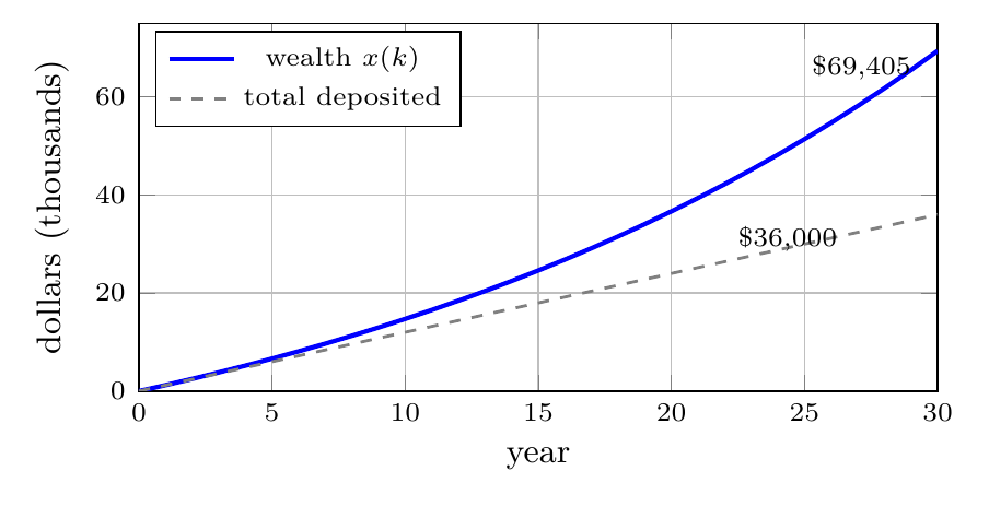
Beginning-of-month deposits: USD 100 monthly for 30 years at a nominal annual rate of 4%, compounded monthly.
The dynamics are what make the difference between USD 36,000 and USD 69,636.29: each month’s wealth feeds back into the next month’s growth.
Open interactive animation · Download animation and source code
Video version
Model properties
A model $y(t) = \mathcal{M}\big(u(t)\big)$ can be classified by how the output depends on the input.
- Memoryless (static) if $y(t)$ depends only on $u(t)$ at the same instant, e.g. $y(t) = \gamma u(t)$.
- Dynamic (with memory) if $y$ at time $t$ depends on input values at other times, e.g. $y(t) = \int_0^t u(\tau)\,d\tau$ or $y(k) = \sum_{i=0}^k u(i)$.
- Causal if $y(t)$ depends on $u(\tau)$ only for $\tau \le t$: the output cannot anticipate the input. All physical systems are causal.
- Acausal (noncausal) if $y(t)$ depends on future inputs $u(\tau)$, $\tau \gt t$. Such models appear in offline signal processing, where the whole record is available.
- Strictly causal if $y(t)$ depends on $u(\tau)$ only for $\tau \lt t$, e.g. the pure delay $y(t) = u(t-10)$.
Linearity and time invariance
Two properties make a model far easier to analyze.
Linearity. $\mathcal{M}$ is linear if it satisfies the superposition property
$$\mathcal{M}\big(\alpha_1 u_1(t) + \alpha_2 u_2(t)\big) = \alpha_1\mathcal{M}\big(u_1(t)\big) + \alpha_2\mathcal{M}\big(u_2(t)\big)$$for any inputs $u_1$, $u_2$ and any real numbers $\alpha_1$, $\alpha_2$.
Time invariance. $\mathcal{M}$ is time-invariant if its properties do not change with time: shifting the input by $T$ just shifts the output by $T$.
Examples:
- $\dot y(t) = Ay(t) + Bu(t)$ is linear and time-invariant (LTI).
- $\dot y(t) = 2y(t) - \sin\big(y(t)\big)u(t)$ is nonlinear, yet time-invariant.
- $\dot y(t) = 2y(t) - t\,\sin\big(y(t)\big)u(t)$ is time-varying: the coefficient $t$ changes the system as time goes on.
Everything in this course, from transfer functions to root loci to Bode plots, relies on the model being LTI. Nonlinear systems are usually handled by linearizing them about an operating point.
“All models are wrong, but some are useful”
The statistician George Box observed that all models are wrong, but some are useful. Models always fall short of the complexities of reality but can still be useful. There are several reasons:
- A dynamic system may simply be too complex to model completely. Consider the neural system of the human brain.
- There are inevitable hardware uncertainties, such as the fatigue of gears or bearings in a car.
- The same design, built many times, varies from unit to unit.
Hard-disk drives illustrate the last point well. Temperature changes and manufacturing variations shift every resonance. The frequency responses of nine drives of the same product line, measured under different conditions, spread out visibly above 5 kHz, and the resulting track-following errors differ from case to case.
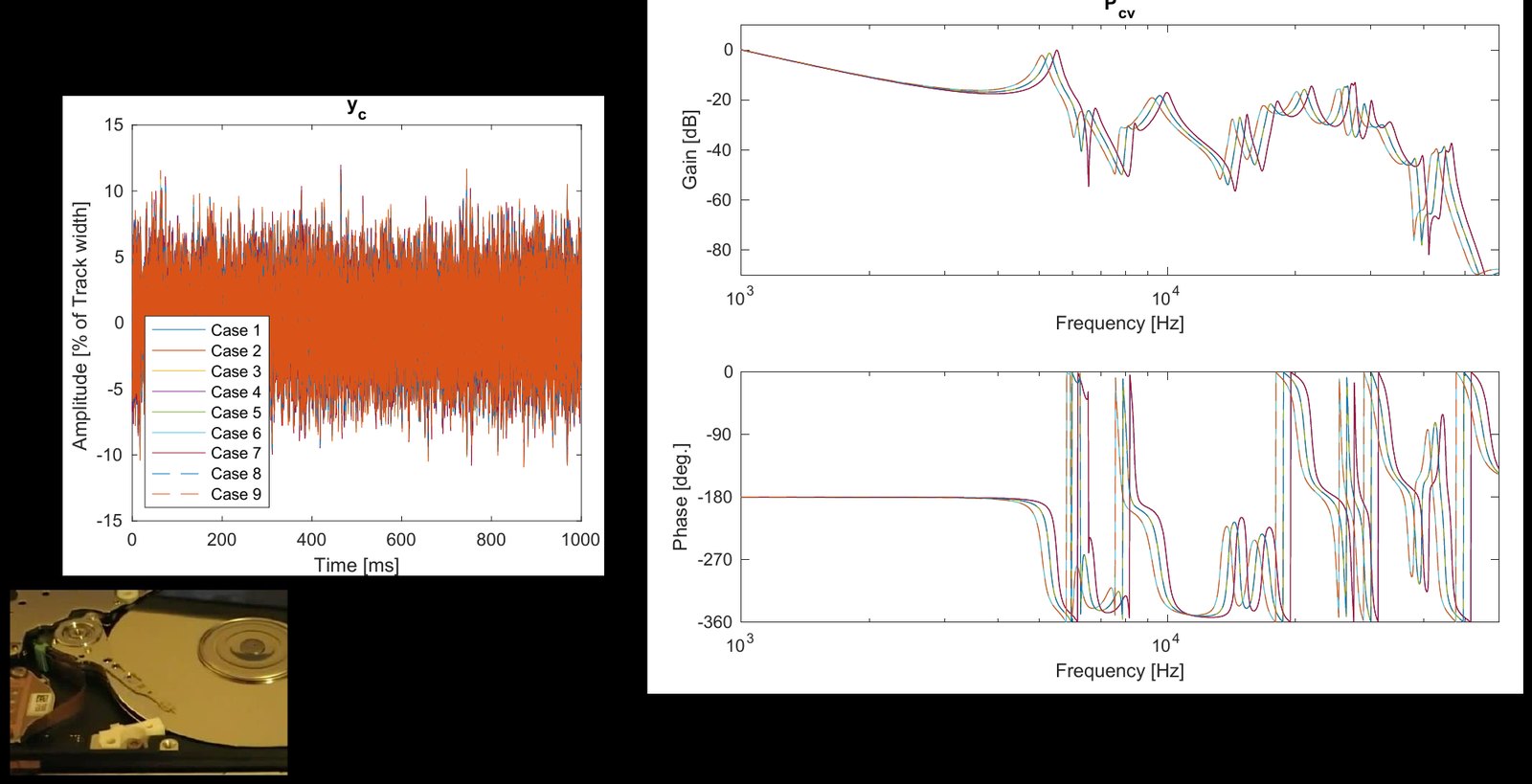
HDDs under perturbation: nine plant variations (right) and the resulting position error (left).
Yet every one of those drives works, because control works: feedback is designed to tolerate the gap between model and reality. This is objective 4 from Lecture 1, robustness to plant uncertainties. Use PyHDD Benchmark, a Python-based framework for magnetic-head positioning control systems in hard disk drives, to explore plant models and controller performance.
Zidong Liu, Yusen Wan, Richard Lu, Amy Santoso, Xiaohai Hu, Thomas Chu, Tianyu Jiang, Guoxiao Guo, Takenori Atsumi, and Xu Chen. “PyHDD benchmark: a python-based framework for magnetic-head positioning control systems in hard disk drives.” 23rd IFAC World Congress, July 2026.
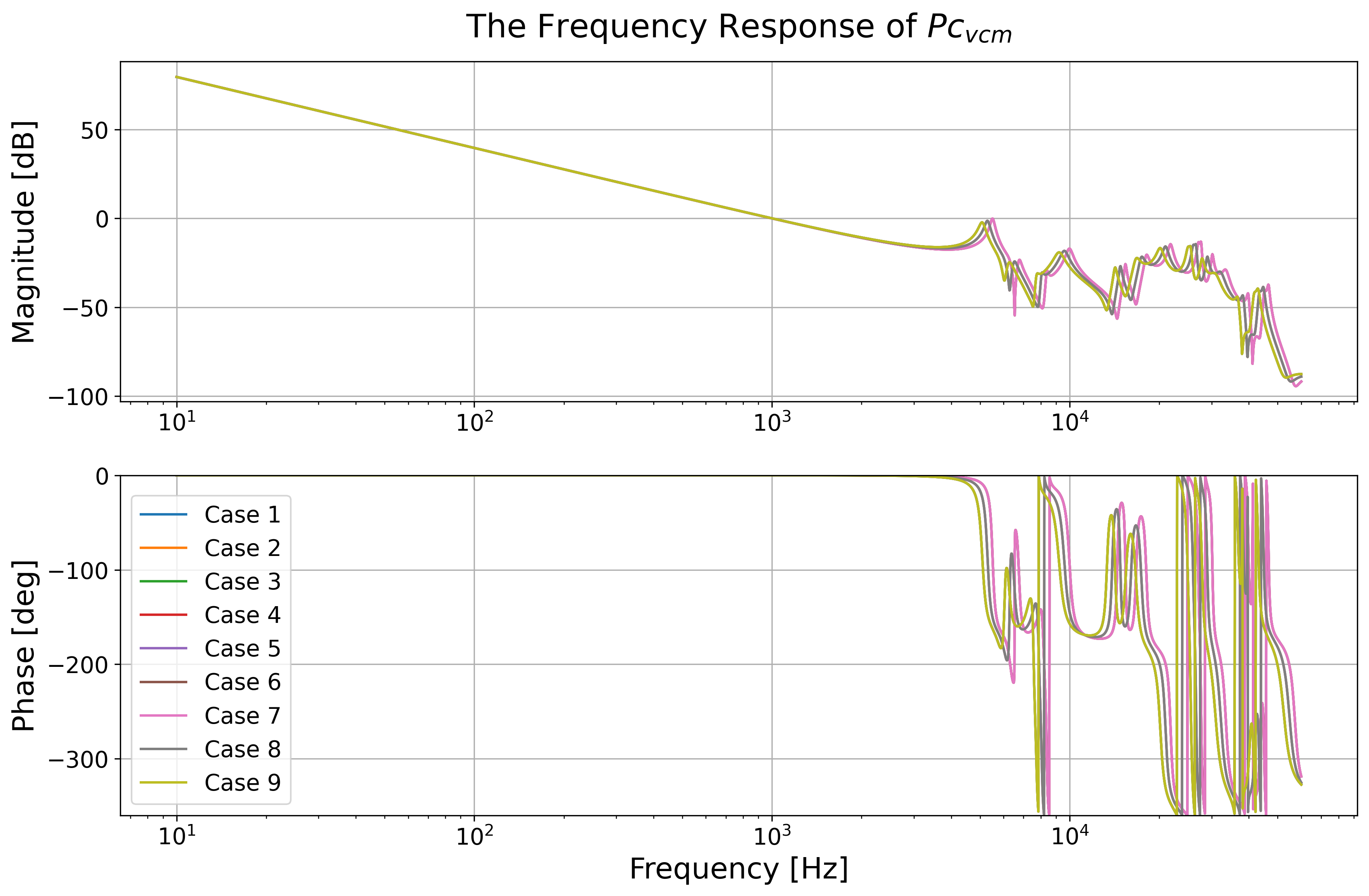
VCM plant frequency responses from PyHDD Benchmark (repository figure 9).
Summary and outlook
- A model lets us simulate and predict, and design model-based controllers.
- Models come from physics (first principles), from data (system identification), or, most often, from both.
- The mass-spring-damper and the HDD actuator lead to second-order ODEs. Resonant modes add more second-order terms in parallel.
- Continuous-time systems are modeled by ODEs, discrete-time systems by difference equations.
- Models can be static or dynamic, and causal, acausal or strictly causal. Linear time-invariant models are the basis of classical control.
- All models are wrong, but some are useful. Feedback makes up for the difference.
An $n$th-order ODE is still awkward to work with directly. The next lecture introduces the tool that turns it into algebra: the Laplace transform.
References
- N. S. Nise, Control Systems Engineering, 6th ed.: §1.4 Analysis and Design Objectives (p. 10); §2.1 Introduction (p. 34); §2.5 Translational Mechanical System Transfer Functions (p. 61); §2.6 Rotational Mechanical System Transfer Functions (p. 69); §2.10 Nonlinearities (p. 88); §2.11 Linearization (p. 89).
- X. Chen and M. Tomizuka, Introduction to Modern Controls, with Illustrations in MATLAB and Python: §2.1 Methods of Modeling (p. 9); §2.2 Continuous-Time Systems (p. 10); §2.3 Discrete-Time Systems (p. 11); §2.5 Example: Hard Disk Drive and Information Storage (p. 14); §2.6 Model Properties (p. 19); §2.7 Nonlinear Systems (p. 20); §2.8 “All Models are Wrong, but Some are Useful” (p. 23).