Lecture 14: Angles of Departure and Arrival
Lecture 13 derived the rules for sketching a root locus. In practice, the rules sometimes leave two or more sketches that look equally plausible: both are symmetric, both start at the poles, and both follow the asymptotes far away. This lecture works through a sequence of board examples in which that happens and shows how a single extra calculation, the angle of departure from a pole (or the angle of arrival at a zero), picks the correct one. Only after the examples do we state the technique in general. Every locus in this lecture is computed exactly; the dashed curves are the tempting but wrong sketches.
Board example 1: two poles on the imaginary axis
Start with the simplest case, $G(s) = \dfrac{1}{s^2+1}$, with poles at $\pm j$ and no zeros.
- Two branches; $n - m = 2$ asymptotes at $\pm90^\circ$.
- The centroid is $\sigma_a = (j - j)/2 = 0$.
The closed-loop characteristic equation $s^2 + 1 + K = 0$ gives $s = \pm j\sqrt{1+K}$: the poles slide along the imaginary axis toward $\pm j\infty$. Nothing is ambiguous here, and every rule agrees. Note the arrows showing the direction of increasing $K$; always draw them.
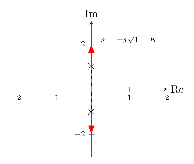
The loop is marginally stable for every $K \gt 0$: proportional feedback alone cannot add damping to an undamped oscillator.
Board example 2: four poles, no zeros
Now take four poles and no zeros,
$$G(s) = \frac{1}{\big((s+1)^2+1\big)\big((s+3)^2+1\big)}, \qquad \text{poles } -1\pm j,\ -3\pm j .$$The asymptote rules give $n - m = 4$ asymptotes at $\pm45^\circ$ and $\pm135^\circ$, centered at the average of the poles, $\sigma_a = (-1 - 1 - 3 - 3)/4 = -2$. There are no real-axis segments, since no poles or zeros are on the real axis.
On the board, a natural first sketch (dashed) lets the poles $-1+j$ and $-3+j$ move toward each other, meet at $-2 + j$, and turn vertically, with the mirror image below. It is symmetric, it starts at the poles, and it ends up heading off to infinity. Is it right?
Check the direction in which the locus leaves $-1 + j$. Place a test point just next to it. Seen from there, the other three poles are at the angles they make with $-1 + j$ itself:
- from $-1 - j$: the vector $2j$, angle $90^\circ$;
- from $-3 + j$: the vector $2$, angle $0^\circ$;
- from $-3 - j$: the vector $2 + 2j$, angle $45^\circ$.
The angle condition $\angle G = -180^\circ$ requires
$$-(90^\circ + 0^\circ + 45^\circ) - \theta_{dep} = -180^\circ \quad\Longrightarrow\quad \theta_{dep} = 45^\circ .$$The branch leaves $-1 + j$ at $45^\circ$, up and to the right, not to the left. The same calculation at $-3 + j$ gives $135^\circ$. In fact the four branches run straight along the asymptotes, as the computed locus shows. The dashed sketch violates the angle condition from the very first step.
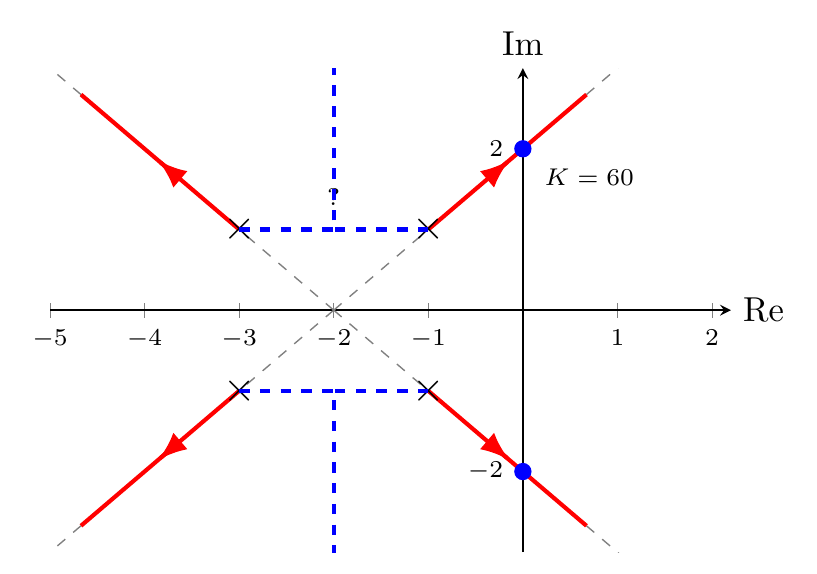
The difference matters. The correct locus crosses the imaginary axis at $\pm2j$. The gain there is the product of the pole distances, $K = \sqrt2\cdot\sqrt{10}\cdot\sqrt{10}\cdot\sqrt{18} = 60$, so the loop is stable only for $0 \lt K \lt 60$. The dashed sketch would have predicted stability for every $K$.
Board example 3: a zero at the origin
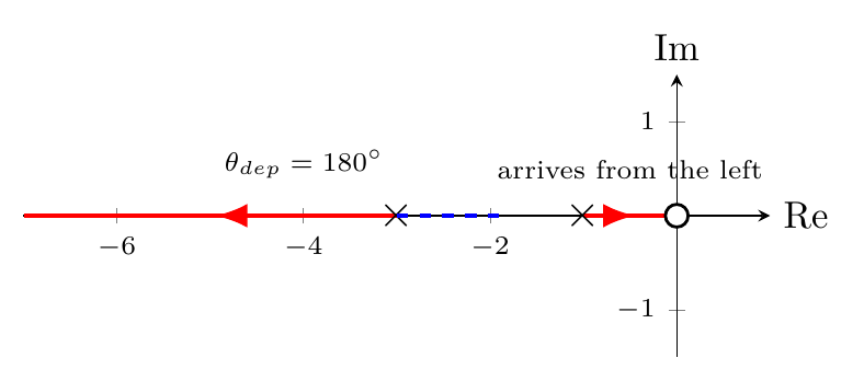
Next consider $G(s) = \dfrac{s}{(s+1)(s+3)}$: a zero at $0$ and poles at $-1$ and $-3$.
The real-axis rule gives the segments $[-1, 0]$ (one pole or zero to the right) and $(-\infty, -3]$ (three to the right). The segment between $-3$ and $-1$ has two to the right, so it is not on the locus. There is $n - m = 1$ asymptote, along $180^\circ$.
Departure from $-3$. Seen from a test point next to $-3$, the zero at $0$ and the pole at $-1$ are both to the right, so the vectors from them to the test point both have angle $180^\circ$. They enter the angle condition with opposite signs and cancel:
$$180^\circ - 180^\circ - \theta_{dep} = \pm180^\circ \quad\Longrightarrow\quad \theta_{dep} = 180^\circ .$$The branch leaves $-3$ to the left, toward $-\infty$. A branch leaving at $0^\circ$ (dashed) looks reasonable on a quick sketch but fails the condition.
Arrival at $0$. The branch from $-1$ must end at the zero. From which side does it arrive? Approaching from the right, every vector (from $0$, $-1$ and $-3$) has angle $0^\circ$, the total is $0^\circ\ne\pm180^\circ$, so this is impossible. Approaching from the left, the vector from the zero has angle $180^\circ$ and the poles contribute $0^\circ$: the condition holds. The branch arrives from the left, along $[-1, 0]$.
Board example 4: when the departure angle decides feasibility
The last board example shows that the departure angle can decide whether a design is possible at all:
$$G(s) = \frac{1}{(s+2)(s^2+4)}, \qquad \text{poles } -2,\ \pm2j .$$The asymptotes are at $60^\circ$, $180^\circ$ and $300^\circ$, centered at $\sigma_a = (-2 + 2j - 2j)/3 = -2/3$, which is in the left half-plane. A quick sketch (dashed) lets the branches from $\pm2j$ first bend left toward the asymptotes. That sketch suggests a range of small gains for which the loop is stable.
Compute the departure angle at $+2j$. Seen from $+2j$, the pole at $-2$ is along $2 + 2j$ (angle $45^\circ$) and the pole at $-2j$ is along $4j$ (angle $90^\circ$):
$$0 - (45^\circ + 90^\circ) - \theta_{dep} = -180^\circ \quad\Longrightarrow\quad \theta_{dep} = 45^\circ .$$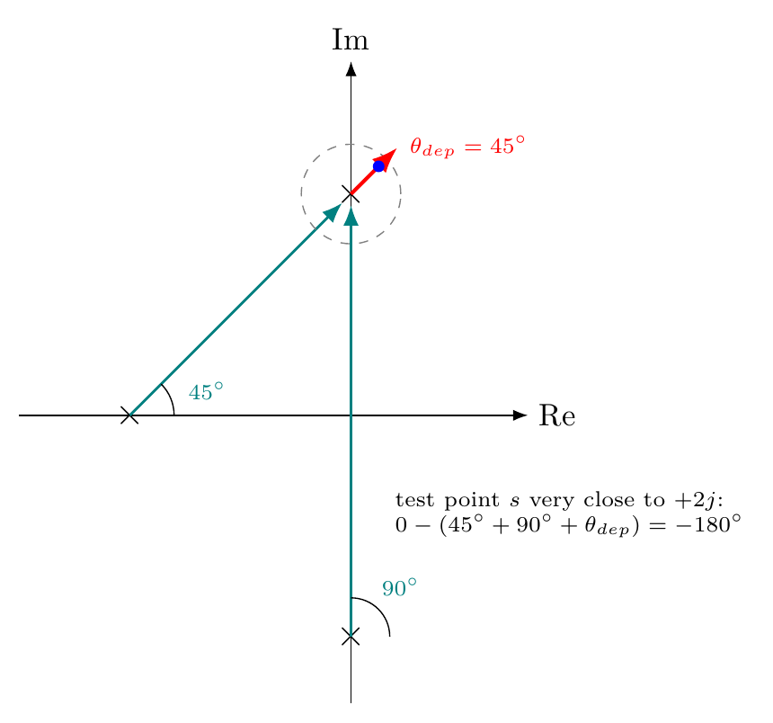
The branch leaves into the right half-plane. For any $K \gt 0$ the closed loop has two unstable poles.
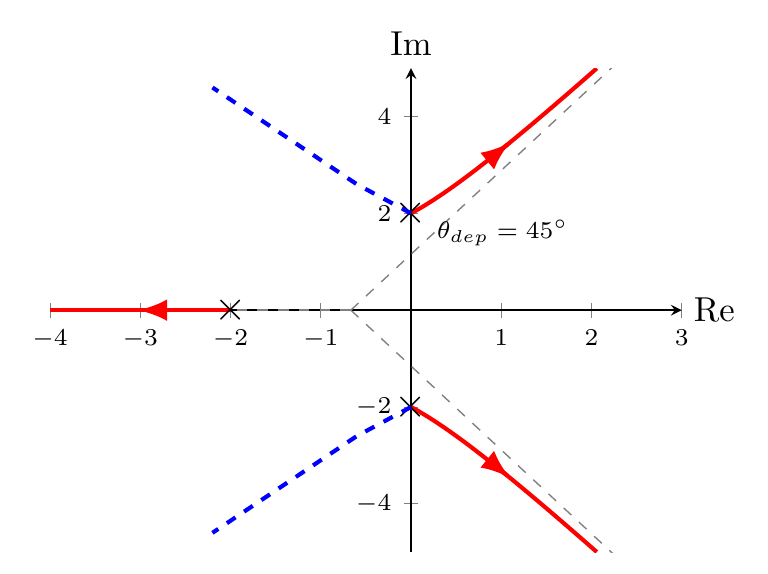
The Routh table of Lecture 10 confirms it. The characteristic polynomial is $s^3 + 2s^2 + 4s + 8 + K$, and the $s^1$ entry of its table is $\big(2\cdot4 - (8+K)\big)/2 = -K/2 \lt 0$ for every $K \gt 0$: two sign changes, two RHP poles. A gain cannot fix this plant; it needs a compensator that adds phase (a zero), the subject of Lectures 17 and 18.
A reminder: asymptotes need branches that go to infinity
One assumption is easy to forget: the asymptote rules describe only the $n - m$ branches that go to infinity. When $n = m$, as for $G(s) = \frac{(s+3)(s+4)}{(s+1)(s+2)}$ in Lecture 13, there are no asymptotes at all, and the shape of the locus is fixed by the start and end points, the real-axis segments and symmetry, and, if needed, by departure and arrival angles.
The technique
All four examples used the same argument. We now state it in general.
The angle condition. Every root-locus rule follows from
$$1 + KG(s) = 0 \iff KG(s) = -1 .$$For $K \gt 0$, a point $s$ is on the locus if and only if $G(s)$ points in the direction of $-1$:
$$\angle G(s) = \sum_j\angle(s - z_j) - \sum_i\angle(s - p_i) = \pm180^\circ\ (\text{mod } 360^\circ).$$The zeros enter with a plus sign and the poles with a minus sign because the phase of a ratio is the phase of the numerator minus the phase of the denominator.
Angle of departure from a pole $p_k$. Place a test point $s$ on a tiny circle around $p_k$. The angles from all the other poles and zeros are essentially the angles from $p_k$ itself. The only unknown is $\angle(s - p_k) = \theta_{dep}$, the direction in which the branch leaves. The angle condition gives
$$\theta_{dep} = \sum_j\angle(p_k - z_j) - \sum_{i\ne k}\angle(p_k - p_i) \pm 180^\circ .$$Angle of arrival at a zero $z_k$. In the same way, with a test point near $z_k$,
$$\theta_{arr} = \sum_i\angle(z_k - p_i) - \sum_{j\ne k}\angle(z_k - z_j) \pm 180^\circ .$$Repeated poles or zeros. If $p_k$ has multiplicity $q$, then $q$ branches leave it, at $q\,\theta_{dep} = (\text{right-hand side}) + 360^\circ(l - 1)$, $l = 1, \ldots, q$: the branches are evenly spaced around the pole.
When to use it. Compute departure angles at every complex pole and arrival angles at every complex zero. Also compute them whenever a real pole or zero leaves two candidate directions, as in board example 3. A procedure that works well at the board:
- Plot the poles and zeros; mark the real-axis segments.
- Compute the asymptotes, if $n \gt m$.
- Compute the departure and arrival angles.
- Only then connect the pieces, with symmetry, and add arrows for increasing $K$.
- If stability is in question, find the $j\omega$ crossing (Routh table) and the gain there.
Summary and outlook
| Rule | Use |
|---|---|
| Symmetry about the real axis | always |
| Real-axis segments to the left of an odd count of real poles and zeros | always |
| Asymptote angles and centroid | only when $n \gt m$ |
| Departure angle from a complex (or ambiguous) pole | decides the branch direction |
| Arrival angle at a zero | decides the approach direction |
| All of the above | come from $\angle G(s) = \pm180^\circ$ |
- A plausible sketch can violate the angle condition; the departure angle catches this immediately.
- In board example 2, the departure angle turns “stable for all $K$” into “stable for $K \lt 60$”; in board example 4, it shows that no gain stabilizes the loop.
The next lecture applies these rules to a realistic motion-control system and shows how a pole that barely affects the transient can still limit the achievable gain.
References
- N. S. Nise, Control Systems Engineering, 6th ed.: §8.3 Properties of the Root Locus (p. 394); §8.4 Sketching the Root Locus (p. 397); §8.5 Refining the Sketch (p. 402), including angles of departure and arrival; §8.6 An Example (p. 411).
- X. Chen, “Essentials of root locus,” topic notes (departure and arrival angles, repeated poles).