Lecture 8: Dominant Pole Analysis
We now understand first- and second-order systems completely. A general system, however, has $n$ poles and $m$ zeros, real or complex:
$$G(s) = \frac{b_m s^m + \dots + b_0}{s^n + a_{n-1}s^{n-1} + \dots + a_0}.$$Two things are new: there are more poles, whose effects combine, and there may be zeros. We treat these one at a time. This lecture keeps the numerator simple and studies how poles combine; the next lecture turns to zeros. The central idea is that of dominant poles: in many systems a few poles govern the response, and the rest can be ignored for the transient.
A real pole plus a complex pair
The simplest case beyond second order adds one real pole to a complex pair:
$$G(s) = \frac{K}{(s+\alpha)\,(s^2 + 2\zeta\omega_n s + \omega_n^2)},\qquad U(s) = \frac1s.$$The partial-fraction expansion follows the same logic as in Lecture 7, with one extra term:
$$Y(s) = \frac{k_1}{s} + \frac{k_2(s+\zeta\omega_n) + k_3\omega_d}{(s+\zeta\omega_n)^2+\omega_d^2} + \frac{k_4}{s+\alpha},$$so that
$$y(t) = k_1 + e^{-\zeta\omega_n t}\bigl(k_5\cos\omega_d t + k_6\sin\omega_d t\bigr) + k_4\,e^{-\alpha t}.$$The coefficients $k_5$ and $k_6$ need not equal $k_2$ and $k_3$, but the structure is what matters. Each pole contributes one mode: the input’s pole at the origin gives a constant, the complex pair a decaying oscillation, and the real pole a decaying exponential.
Plotting the poles in the complex plane builds intuition for how each mode behaves:
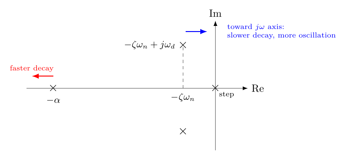
A complex pair that moves toward the imaginary axis decays more slowly and oscillates more, because it approaches the stability boundary. A pole that moves further left decays faster.
When the real pole is far away
Consider the extreme case in which $-\alpha$ lies far to the left of the complex pair. Then $e^{-\alpha t}$ dies out almost immediately, and what remains is essentially the second-order response of Lecture 7. The pole at $-\alpha$ has almost no visible effect on the transient.
One caution is essential. The fast pole does not affect the shape of the transient, but it does affect the steady-state level. By the final value theorem,
$$y(\infty) = \lim_{s\to0} s\,Y(s) = \frac{K}{\alpha\,\omega_n^2}.$$The initial value is still $y(0) = \lim_{s\to\infty} sY(s) = 0$. In practice, the response starts out slightly differently from a pure second-order response and very soon looks like one, but it settles at a level that includes the factor $1/\alpha$.
The rule of thumb
How far is “far enough”? A widely used rule of thumb says:
If the real pole lies at least five times further left than the real part of the complex pair, $\alpha \ge 5\,\zeta\omega_n$, its transient is negligible and $y(t)$ is approximately a second-order response.
The poles closest to the imaginary axis then govern the response; they are the dominant poles. The comparison below shows responses scaled to the same final value. At $\alpha = 5\zeta\omega_n$ the third-order response nearly matches the second-order one; at $\alpha = \zeta\omega_n$ it does not:
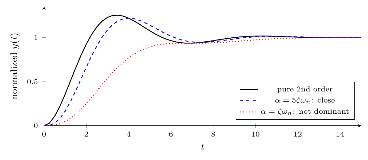
When the real pole is not far away, the response is a genuine superposition of modes, and the second-order formulas for overshoot and peak time no longer apply.
Generalization
The same reasoning extends to any number of poles. Additional real poles add exponential modes; those far from the imaginary axis can be dropped for the transient but must be kept when computing the steady-state value. Additional complex pairs add damped oscillations:
$$y(t) = k_0 + e^{-\zeta_1\omega_1 t}\bigl(A_1\cos\omega_{d1}t + B_1\sin\omega_{d1}t\bigr) + e^{-\zeta_2\omega_2 t}\bigl(A_2\cos\omega_{d2}t + B_2\sin\omega_{d2}t\bigr) + \cdots$$The same rule applies: if $\zeta_2\omega_2 \ge 5\,\zeta_1\omega_1$, the first pair dominates.
Summary and outlook
- Every pole is a mode, and the transient is a superposition of modes.
- The poles closest to the imaginary axis dominate. Poles at least five times further left can be ignored for the transient.
- The final value must always be computed from the full transfer function.
So far the numerators have been constants. The next lecture adds a zero and discovers that zeros can reshape the transient dramatically, sometimes making the response start in the wrong direction.
References
- N. S. Nise, Control Systems Engineering, 6th ed.: §4.7 System Response with Additional Poles (p. 186).
- X. Chen and M. Tomizuka, Introduction to Modern Controls, with Illustrations in MATLAB and Python: §3.2 Inverse Laplace Transform and Partial Fraction Expansion (p. 39).