2. A Stochastic DTS

A primer: Part 2

Author

Affiliation

University of Washington

In the previous vignette, we presented a deterministic discrete-time system (DTS). Here, we develop a system with all the same rules, but updating is stochastic — the outcome relies on the value of a random number.

If we followed individuals in a population that followed the simple rules described in the previous set of equations, then each individual would be either infected or uninfected, and we could count them up. In the deterministic DTS we just looked at, the variables can take on any real value. No one can be half-infected, so what do they mean? For now, we can think of those values as expectations, but what if we wanted to follow individuals over time? To do that, we need to be able to deal with random changes in an individual’s status from day to day. We need a new kind of model.

Setting aside the problems that get introduced by observing (e.g. sampling) populations for the moment — we’ll pretend we’re omniscient — we would find random changes occurring:

individual humans would be switching states every day at random: from infected to uninfected and back;
individual mosquitoes would be dying at random: infected mosquitoes would get replaced by uninfected mosquitoes, and uninfected mosquitoes would be blood feeding and getting infected if they blood fed on an infected (and infectious) human.

The world really has a random component to it. It is not deterministic but stochastic.

In the deterministic models in the previous vignette called ross_diffs_1 and ross_dts_2, the values of each variable at each point in time were specified exactly by the equations, the rules for updating the variables each day. The values of the variables were proportions, which is related to the metric prevalence. In these models, the variables asymptotically approach a steady state. Once at the steady state, the fractions infected would never change.

In models with stochasticity, we could use the same exact rules to specify what is expected to happen, but we must draw a random number to determine the values of the variables. To do this, we want to be working with the counting numbers – the number of humans in a population and the number of those humans who are infected; and the number of mosquitoes in a population, and the number of those mosquitoes who are infected. The variability in the values of our variables over time due to the random component of parasite infection dynamics – also called the parasite demographics – would be called demographic stochasticity. The model has some things in common with the ones we described above: the model doesn’t have a steady state, but there is something like a steady state that the variables fluctuate around. We’ll call it an attractor. The variables are always pulled towards the attractor, but the values of the variables are constantly changing around it.

In a real study, we can pretend to be omniscient but pretending doesn’t make it so. We’ll deal with that later.

Parameters – We can use the same parameters as before, but we need to name two new parameters:

\(M\) is the number of mosquitoes: it is a counting number
\(H\) is the number of humans; it is a counting number

Otherwise we use the same parameters as we did before.

# The parameters, as a list 
ross_sdts_par = list(
  M = 50,   # The number of mosquitoes 
  H = 100,   # The number of humans 
  s = 1/200, # The fraction of infections that clear each day
  u = 1/12,  # The fraction of mosquitoes that die each day
  a = 1/4   # The fraction of mosquitoes that blood feed on a human each day
)
ross_sdts_par$m = with(ross_sdts_par, M/H)

Variables

In the stochastic model, the variables are counting numbers, not fractions:

\(Y \leq M\) is the number of infected mosquitoes: \(Y\) is a counting number
\(X \leq H\) is the number of infected humans: \(X\) is a counting number

It is easy enough to define prevalence:

\(x = X/H\) is malaria prevalence in humans; the fraction of humans infected
\(y = Y/M\) is malaria prevalence in mosquitoes; the fraction of mosquitoes infected

Equations

Now we have got to describe a stochastic process. Each individual changes state with some probability. Each one is a Bernoulli random variable, and the appropriate proability mass function is the binomial model. In R, we use the built-in function rbinom(1, N, p) to draw one random variable on \(N\) individuals that remains in the same state with probability \(p\).

In each step, there are four possible changes, depending on the states:

\(X\) — if humans are infected today, they might lose infection. An infection is lost with probability \(s\), so the fraction that remain infected is \(1-s.\) The number that remains infected is rbinom(1, X, 1-s).
\(H-X\) — if humans are uninfected today, they might get infected. The probability of getting infected is called the daily attack rate. The expected number of infected bites is \(aY/H\), and if we use the Poisson to model the distribution of bites per person, then the attack rate is \(1-e^{-aY/H}\). The number that remains ends up infected is rbinom(1, H-X, ar).
\(Y\) — if mosquitoes are infected today, they might die. The fraction dying is \(u\), so the number of surviving infected mosquitoes is rbinom(1, X, 1-s).
\(H-Y\) — if mosquitoes are uninfected today, they might get infected. To get infected, a mosquito must blood feed on an infected human, so the fraction getting infected is \(aX/H\). The number that gets infected is rbinom(1, H-Y, a X/H).

The rule for updating the number of infected humans and mosquitoes is thus:

\[\begin{equation} \begin{array}{rl} X_{t+1} &= \mbox{Binom}(X, 1-s) + \mbox{Binom}(H-X, 1-e^{-a Y/H}) \\ Y_{t+1} &= \mbox{Binom}(Y, 1-u) + \mbox{Binom}(M-Y, aX/H) \\ \end{array} \end{equation}\]

The following implements this as R code:

# XY      - a vector of the form c(t, X, Y) 
# params  - the parameters, as a list 
ross_sdts = function(XY, params){
  with(as.list(XY), 
    with(params,{
      ar = 1 - exp(-a*Y/H)
      Xn = rbinom(1, X, 1-s) + rbinom(1, H-X, ar)  
      Yn = rbinom(1, Y, 1-u) + rbinom(1, M-Y, a*X/H)  
      t=t+1
      return(c(t=t, X=Xn, Y=Yn))
}))}

We write a wrapper that solves it:

# INPUTS
# pars - the parameters, as a list 
# X0   - the initial number of infected humans
# Y0   - the initial number of infected mosquitoes 
# t0   - the initial value of t
# tmax - the last value of t 
#
# OUTPUTS
# the values of the variables over time, as a list 
sim_ross_sdts = function(pars, X0=2, Y0 = 1, t0=0, tmax=100){
   XY = c(t=t0, X=X0, Y=Y0) 
   XY_t = XY 
   for(t in (t0+1):tmax){
     XY = ross_sdts(XY, pars)
     XY_t = rbind(XY_t, XY)
   }
   X=XY_t[,2] 
   Y=XY_t[,3]
   x=X/pars$H 
   y=Y/pars$M 
   return(list(time=XY_t[,1], x=x, y=y, X=X, Y=Y, last = XY)) 
}

We can write another function that plots the equations (i.e. that iteratively computes and stores the values) over some time interval:

# INPUTS
# XY_t - a list with elements named x, y, and time
# type - plot type:  "l" or "p" or "b"
# lty  - lty  
# add  - if TRUE, add to existing plot 
plot_XY = function(XY_t, type="l", lty=1, add= FALSE){with(XY_t,{
  if(add == FALSE) 
  plot(time, X, type = "n", ylim = range(0, X, Y), ylab = "Number Infected", xlab = "Time")
  lines(time, X, type=type, lty=lty, col="darkgreen", pch =15)
  lines(time, Y, type=type, lty=lty, col="darkorange", pch =19)
  text(0, 0.9*max(X,Y), "X", col = "darkgreen", pos=4) 
  text(0, 0.8*max(X,Y), "Y", col = "darkorange", pos=4) 
})}

A useful feature of R is the ability to replicate any particular sequence of random numbers by setting a seed. This also makes it easy to write a book knowing what the random number sequence will be.

set.seed(253)
XYt <- sim_ross_sdts(ross_sdts_par, tmax=1000)

plot_XY(XYt)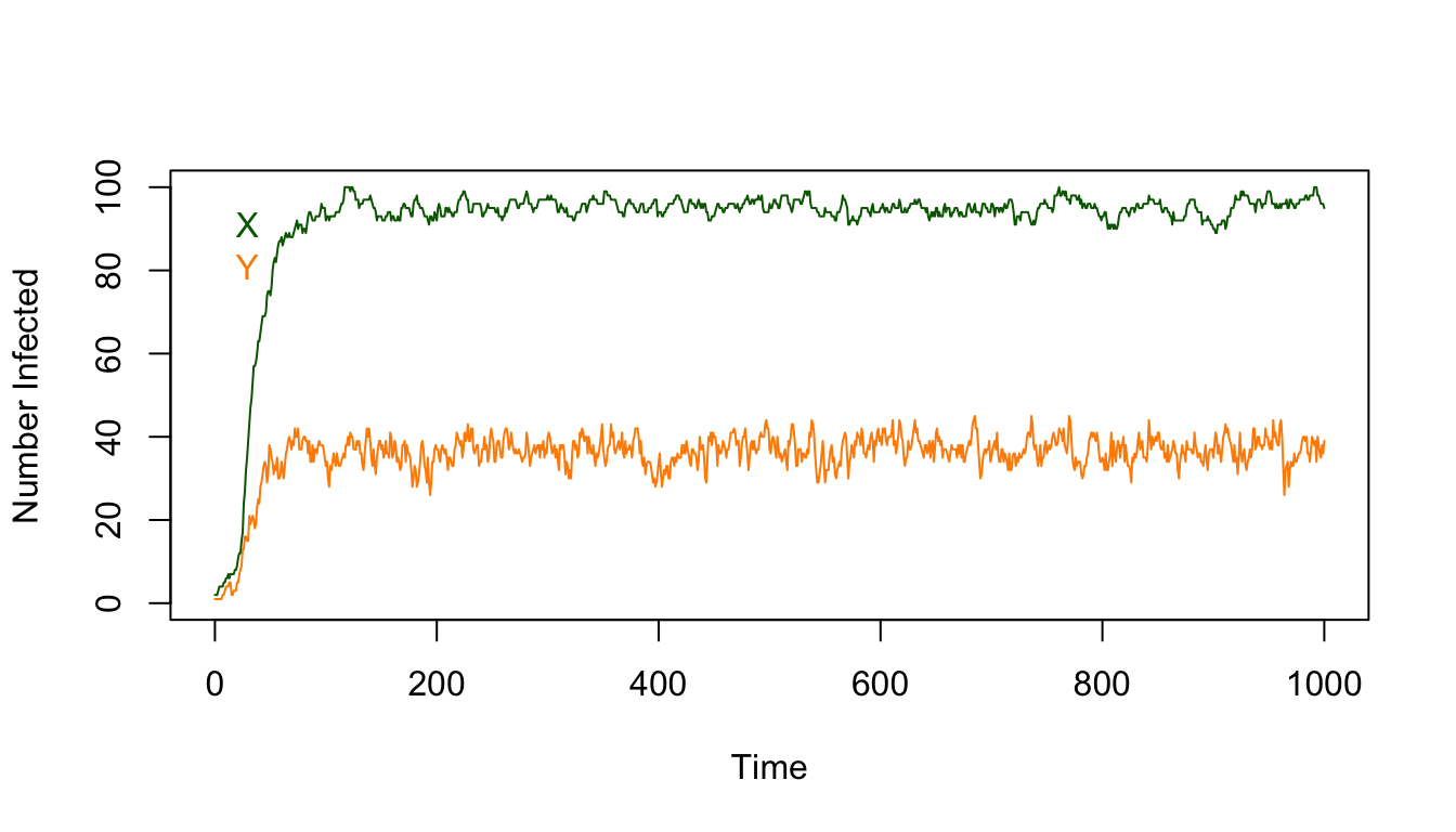

Once we’re close to the steady state, some time after the first 100 days, we can compute the mean:

Xdist= with(XYt, X[-c(1:100)]) 
Ydist= with(XYt, Y[-c(1:100)]) 
mX = mean(Xdist)
mY = mean(Ydist) 
c(X=mX, Y=mY)

       X        Y 
95.09989 36.76027

This can be visualized as a histogram:

par(mfrow=c(1,2))
hist(Xdist,  xlab = "x", main = "X, for t>100")
segments(mX, 0, mX, 250, lwd=4, col = "darkgreen")
hist(Ydist, 15, xlab = "y", main = "Y, for t>100")
segments(mY, 0, mY, 200, lwd=4, col = "darkorange")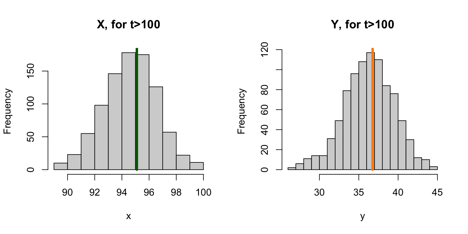

Since we can compute prevalence, we can plot it out:

plot_xy(XYt)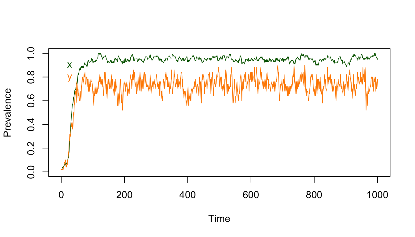

xdist= with(XYt, x[-c(1:100)]) 
ydist= with(XYt, y[-c(1:100)]) 
mx = mean(xdist)
my = mean(ydist)
c(x=mx, y=my)

        x         y 
0.9509989 0.7352053

par(mfrow=c(1,2))
hist(xdist,  xlab = "x", main = "x, for t>100")
segments(mx, 0, mx, 250, lwd=4, col = "darkgreen")
hist(ydist, 15, xlab = "y", main = "y, for t>100")
segments(my, 0, my, 200, lwd=4, col = "darkorange")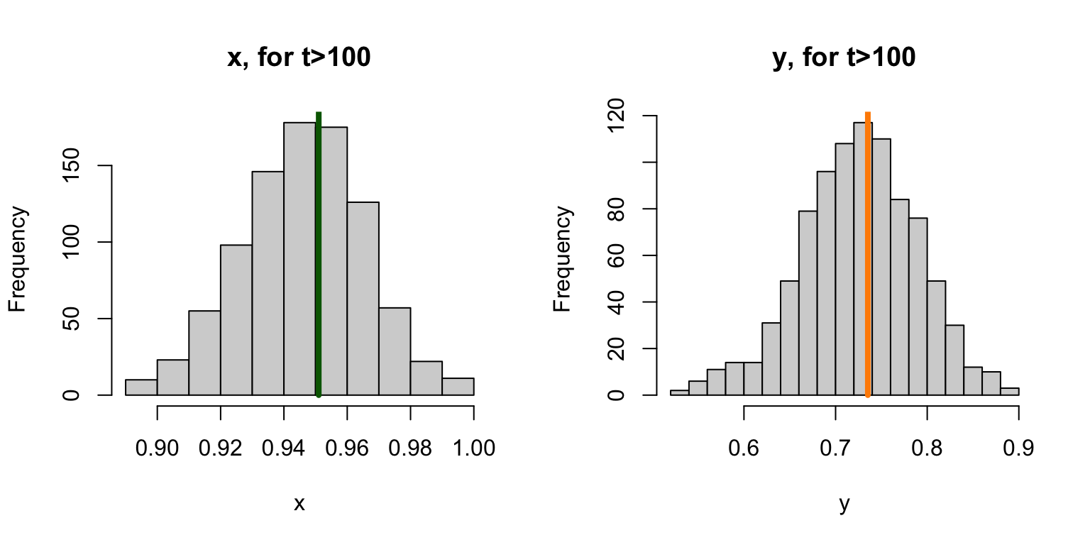

The system still tends towards a point – we’ll call it an attractor and not a steady state. The values of \(X\) and \(Y\) (or of \(x\) and \(y\)) fluctuate around that steady state. Since the counting number values get repeated, we can illustrate what the cloud looks like by jittering the locations of the points:

with(XYt,{
  ix = which(time>100)
  plot(jitter(X[ix],1.5), jitter(Y[ix],1.5), xlab = "X", ylab = "Y", cex=0.2)
}) 
points(mX, mY, col = "darkred", pch = 8, cex =3)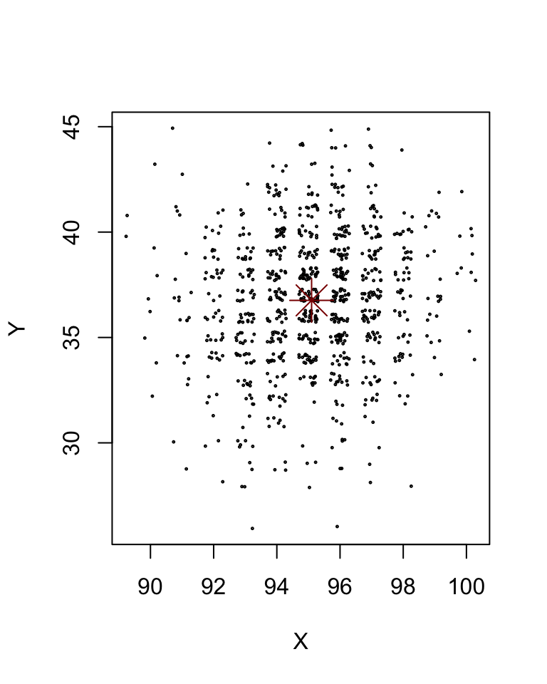

We note that mean prevalence is very close to the steady state of the deterministic system with the same parameter values:

c(mx, my) - ross_dts_steady_1(ross_sdts_par)

           x            y 
 0.002280941 -0.004794673

An important feature of stochastic systems is that it is possible for the parasite to randomly fade out, if at any time \(X=Y=0.\) This is something we’d like to take a bit more time computing.