
VCmatrix = matrix(c(2, 0.3, .5, 1), 2, 2)
VCmatrix
[,1] [,2]
[1,] 2.0 0.5
[2,] 0.3 1.0Vectorial Capacity in Metapopulation Models
The simple formula for VC describes potential malaria transmission by mosquitoes. With spatial dynamics, the concept of VC can be extended into a form that is useful for understanding the effects of targeting interventions spatially. Here, we define vectorial capacity for autonomouos metapopulation models.
See Related for links to closely related vignettes.
In patch-based spatial models, also known as meta-population models, we define two closely related concepts:
Patch VC or \(V,\) a vector of length \(N_p\) — the number of infectious bites that would arise from all the mosquitoes blood feeding in a single patch on a single fully infectious human on a single day; and
The VC Matrix or \([V]\) — how many infectious bites would arise in every patch from all the mosquitoes blood feeding in each patch on a single fully infectious human on a single day, where
\[V = 1 \cdot [V]\]
In a two patch model, a VC matrix is:
VCmatrix = matrix(c(2, 0.3, .5, 1), 2, 2)
VCmatrix [,1] [,2]
[1,] 2.0 0.5
[2,] 0.3 1.0The number of infectious bites arising from each patch, per person, per day, is:
Vvector = c(1,1) %*% VCmatrix
Vvector
[,1] [,2]
[1,] 2.3 1.5At the steady state, the number of infectious bites arriving in each patch, per person, per day, is:
VCmatrix %*% c(1,1) [,1]
[1,] 2.5
[2,] 1.3In a picture:
clrs = c("darkred", "darkblue")
plot_connectivity_sankey(VCmatrix, clrs =clrs)
We can plot the same information spatially, letting the width of the circle represent the amount that stays, and the with of the arrows the flow to other
plot_connectivity_graph(VCmatrix, clrs =clrs, scl=2.5)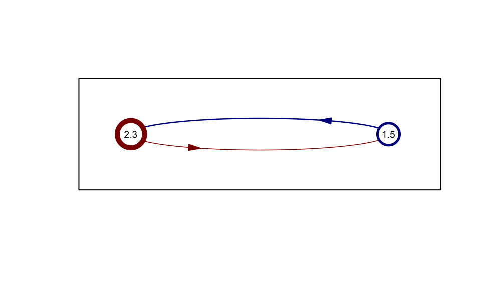
Formulas for the VC matrix are model dependent, but since an example is useful, we will derive a formula to compute the VC using the the spatial analogue of Macdonald’s model.
To compute the VC matrix, we need the mosquito demographic matrix \(\Omega\) that plays the same role as mosquito mortality, but in this case it includes mortality and dispersal.
In the model for mosquito ecology, we get:
\[ \frac{d\vec M}{dt} = \vec \Lambda - \Omega \cdot \vec M \] To model changes in the density of infected mosquitoes, we get:
\[\frac{d \vec Y}{dt} = fq\kappa (M-Y) - \Omega \cdot \vec Y\]
The model for infectious mosquitoes incorporates a delay (the subscript \(\tau\) denotes the value of a variable at time \(t-\tau\)):
\[\frac {d \vec Z}{dt} = e^{-\Omega \tau} \cdot fq\kappa (M_\tau -Y_\tau) - \Omega \cdot \vec Z\]
We can now use the framework to compute the VC. The total biting per patch, \(B\) is
\[fqM\]
We note, for interest, that:
\[\bar M = \Omega^{-1} \cdot \vec \Lambda\] We can understand \(\Omega^{-1}\) as a measure of time spent by the mosquitoes emerging from one patch in every other patch:
\[\Omega = \int_0^\infty e^{-\Omega t} dt\] so the number if human blood meals per mosquito, summed over the lifespan of a mosquito, is:
\[[s] = fq \Omega^{-1}\]
mosquito survival and dispersal through the EIP
\[\Upsilon = e^{-\Omega \tau}\]
To get the patch HBR, we divide total biting by availability \(W\) \[\frac B W\]
Now we can write:
\[V = fq \Omega^{-1} \cdot e^{-\Omega \tau} \cdot \frac{fq\bar M}W = [s] \cdot \Upsilon \cdot \frac{B}{W} \] and (remembering that the order is reversed for matrix operations):
\[[V] = fq \Omega^{-1} \cdot e^{-\Omega \tau} \cdot \left[\left<\frac{fq\bar M}W \right>\right] = [s] \cdot \Upsilon \cdot \left[\left< \frac{B}{W} \right>\right]\]
Average vectorial capacity for the system is:
\[ \frac{\sum fqM} H \]