
# Initial Conditions at a point in time, as a Named Vector
xy = c(t=0, x=0.01, y=0.001)
xy
t x y
0.000 0.010 0.001 A Primer: Part 1
Here, we present a basic, deterministic model for daily malaria dynamics: it is called a discrete time system (DTS). This vignette is a basic introduction: it assumes only that the reader is familiar with basic mathematics. We will, however, start with the basics: we discuss the parts of a model, and we walk through the process of solving models.
We are interested in understanding malaria in populations. Malaria parasites are transmitted by mosquitoes through blood feeding: infectious mosquitoes bite and infect humans; and parasites in the blood of infectious humans are taken up by mosquitoes in the blood meal, infecting a mosquito. After becoming infected, humans can remain infectious for several months. After becoming infected, a mosquito remains infectious until it dies.
We want to write down some equations that represent this process — infection incidents and clearance events in humans and mosquitoes — in terms that we can understand. The process are framed in terms of individuals, but we are tracking the prevalence of infection with malaria parasites in humans and mosquitoes changes over time.
Here, we will describe the daily dynamics of malaria in populations using very basic mathematics: the resulting dynamical system is called a discrete time system. The mathematics are simple enough to be implemented on spreadsheets. Some people find it easier to understand stochastic equations first: we do that in the next vignette. If it helps, you can go back and forth.
The discrete time models ross_diffs_1 and ross_dts_2 have been implemented in a Google Sheet.
We start by introducing models: we describe the parts of the model first and the equations last. The parts of a model are called parameters and variables. To solve the model, we will need initial conditions for the variables. As we go, we will also write R code that implements the model and that solves it. In writing the code, we will adopt some conventions that we can use to help us write good code.
Variables are quantities that describe the state of a system. One variable in this model is time in days, denoted \(t.\) The dependent variables are the quantities that we want to compute: in this case, we compute them every day. Time is marching forward, unaffected by the dependent variables, so we call it the independent variable.
In this model, there are two dependent variables: the proportion of humans and mosquitoes that are infected at each point in time. Since it is a discrete time system, the values of the variables are defined only at integer values of \(t.\) We define the variables as follows:
let \(t\) represent time, in days;
let \(x_t\) be the fraction of people who are infected at time \(t,\) and \(0 \leq x_t \leq 1;\)
let \(y_t\) be the fraction of mosquitoes who are infected at time \(t,\) \(0 \leq y_t \leq 1.\)
Another term for the fraction of a population that infected with parasites is prevalence.
Initial Conditions are the values of the variables at one point in time. Since the values of our variables in the next time step (at time \(t+1\)) depend on their values now (at time \(t\)), we can’t really compute anything specific unless we specify the values of the variables at one point in time. Having set one set of values, we can use the equations to compute the rest.
The initial conditions specify the values of all our variables at the beginning of the simulation. By convention, this is usually at time \(t=0,\) but we could also specify their values at any other point in time.
We can now begin to write R code to set up the objects so we can compute them. We set these initial values to be small:
# Initial Conditions at a point in time, as a Named Vector
xy = c(t=0, x=0.01, y=0.001)
xy t x y
0.000 0.010 0.001 In R, this object xy is called a named vector. The names that appear above the numbrers are carried along but they don’t affect the values of any computation done with xy. It is also useful that the names often get inherited (but not always). The names can be used as names using the function as.list() or data.frame().
as.list(xy)$x[1] 0.01When combined with the with() function, we can create a context where we can call them by name:
with(as.list(xy), x) [1] 0.01This code has adopted the convention of using named vectors so that we can write functions in a way that is easy to read. It also makes it easier to deal with the model outputs.
Parameters are quantities – rates, numbers, or probabilities – that describe some part of the process. Unlike variables, parameter values are chosen outside of a model and passed to it. In ross_diffs_1, these parameters are constant. Since they are constant, we call this an autonomous system of equations. In other models, we could have parameter values that change over time: if so, the system would be called non-autonomous.
The parameters in this model define changes in prevalence: the fraction of humans that clear an infection each day; the fraction of infected mosquitoes that die; and blood feeding and infection.
Let \(s\) denote the fraction of people who clear infections after one day; \(0 < s < 1.\)
Let \(u\) denote the fraction of mosquitoes who die in one day; \(0 < u < 1.\)
Let \(a\) denote the fraction of mosquitoes who blood feed on a human in a day; \(0 < a < 1.\)
Let \(m\) denote the number of mosquitoes per human; \(m \geq 0.\)
# INPUTS
# s - The fraction of infections that clear each day
# u - The fraction of mosquitoes that die each day
# a - The fraction of mosquitoes that blood feed on a human each day
# m - The number of mosquitoes per human
#
# OUTPUTS
# a list with the parameter values by name
ross_dts_makepars = function(
  s = 1/200,
  u = 1/10,
  a = 1/4,
  m = 2
){
  list(s=s, u=u, a=a, m=m)
}
ross_dts_par = ross_dts_makepars()Equations describe dynamic changes in the variables over time. In this case, the process is described by a system of coupled difference equations.
Finally, we put all this together into a mathematical statement that has translated the description of a process, that are describe the process.
\[ \begin{array}{rl} x_{t+1} &= x_t - s x_t + m a y_t (1-x_t) \\ y_{t+1} &= y_t - u y_t + a x_t (1 - y_t) \\ \end{array} \tag{1}\]
We could rewrite the equations to make it easier to interpret them.
\[ \begin{array}{rl} x_{t+1} - x_t &= - s x_t + m a y_t (1-x_t) \\ y_{t+1} - y_t &= - u y_t + a x_t (1 - y_t) \\ \end{array} \tag{2}\]
In this alternative way of writing down the equations, the left hand side is interpreted as the daily change, and the terms on the right hand side describes those changes. The RHS has four terms:
\(- s x_t\) – is a decrease in the prevalence of human malaria infections caused by clearance of human infections: the fraction of humans who are infected is \(x_t\); a fraction \(s\) clears infections each day.
\(+ may_t (1-x_t)\) – is an increase in the prevalence of human malaria infections caused by the bites of infectious mosquitoes: the fraction of humans who are not infected is \(1-x_t\); a fraction \(m a y_t\) gets infected.
\(-u y_t\) – is a decrease in the prevalence of mosquito malaria infections caused by mosquito mortality: the fraction of mosquitoes who are infected is \(y_t\); a fraction \(u\) die.
\(+ a x_t (1-y_t)\) – is an increase in the prevalence of mosquito malaria infections caused blood feeding on an infected human: the fraction of mosquitoes who are not infected is \(1-y_t\); a fraction \(a x_t\) blood feeds on an infected human and gets infected.
To foreshadow something we will address in sub-section @ref(dtsRoss2), if \(may_t >1,\) then it is not a proportion, and the equations don’t make sense.
To update the variables, we write a function in R. Since we will be developing a lot of functions and models, we adopt a simple naming convention: since it was developed by Ross, we attach the stem ross; since this is a discrete time system, we attach the suffix dts; we might want to generate other variants, so we append a number. The function is thus called ross_diffs_1.
# INPUTS
# xy     - current variables, as a named vector
# params - the parameters, as a list
#
# OUTPUTS
# the updated values of the variables, as a named vector

ross_diffs_1 = function(xy, params){
  with(as.list(xy),
    with(params,{
      xn = x - s*x + m*a*y*(1-x)
      yn = y - u*y + a*x*(1-y)
      return(c(t=t+1, x=xn, y=yn))
    })
  )
}With the R code we developed, we can solve the equations, which involves computing the values of the variables iteratively. Since the values of the variables change, we create another object xy_t that we can use to store the values of computed variables over time.
# xy_t stores the values of the variables
xy_t = xy
xy_t
t x y
0.000 0.010 0.001 We iterate in two steps. First, we compute the values.
# Compute
xy = ross_diffs_1(xy, ross_dts_par)
Since we initialized the system at time \(t=0,\) the following computes the values of the parameters at time \(t=1.\) We can take a peak at the values we computed:
# Print to screen
print(xy)
t x y
1.0000000 0.0104450 0.0033975 Next, we store the values using rbind
# Store
xy_t = rbind(xy_t, xy)
We can take a peak:
# Print to screen
print(xy_t)
t x y
xy_t 0 0.010000 0.0010000
xy 1 0.010445 0.0033975We can iterate over many time steps, each time storing the values:
# Iterate to compute the values as they change over time
for(t in 2:40){
  xy = ross_diffs_1(xy, ross_dts_par)
  xy_t = rbind(xy_t, xy)
}
We can look at the last few values, the values of \(t,\) \(x\) and \(y\) are stored in columns:
print(tail(xy_t, 3)) t x y
xy 38 0.9857389 0.7104755
xy 39 0.9858763 0.7107768
xy 40 0.9859663 0.7109837As we can see, the values are changing a little at the end.
Notice that after 40 days, the values of \(x\) and \(y\) appear to be approaching some value asymptotically. This is an important feature of these systems, one that we would like to understand and explore a bit more in the following sections.
The discrete time model ross_diffs_1 can be implemented in a spreadsheet. We did one as a Google Sheet.
The fact that our variables asymptotically approach some values over time is an important feature of dynamical systems, so we would like to do some analysis to understand it better. If we look at Eq. Equation 2, we can understand why. In this model, there is no change when the proportion of humans becoming infected is equal to the proportion clearing infections; and the proportion of mosquitoes becoming infected is equal to the proportion dying.
In the following, we compute how much the system is changing over time. We can simply iterate once and compare the differences. After iterating 40 times, the differences are very small:
# The last value is still stored as xy; the [-1] omits t
xy[-1] - ross_diffs_1(xy, ross_dts_par)[-1]
x y
-5.903348e-05 -1.417083e-04 If we iterate another hundred days and check again, the differences have gotten even smaller:
for(i in 41:140){
  xy = ross_diffs_1(xy, ross_dts_par)
  xy_t = rbind(xy_t, xy)
}
xy[-1] - ross_diffs_1(xy, ross_dts_par)[-1]
x y
0 0 After simulating, the variables reach a steady state, where asymptotically \(x_{t+1} = x_t\) and \(y_{t+1} = y_t\).
A steady state occurs when there is no daily change, so \[x_{t+1} - x_t = 0\] and \[y_{t+1} - y_t = 0.\] We can figure out the steady state values are by substituting \[x_{t+1} = x_t = x\] and \[y_{t+1} = y_t = y\] into Eq.Equation 2 and then solving for \(x\) and \(y\). After cancelling and rearranging, we get:
\[ \begin{array}{rl} m a y (1-x) &= s x \\ a x (1 - y) &= u y\\ \end{array} \tag{3}\]
Equation 3 says: the proportion of humans becoming infected is equal to the proportion clearing infections; and the proportion of mosquitoes becoming infected is equal to the proportion dying.
The most obvious solution to these equations is \(x=y=0,\) when there is no malaria. We call it the disease-free steady state. A disease-free equilibrium makes sense, since if we start with no infected mosquitoes or infected humans in this deterministic model, there can never be any.
There is another solution where malaria is present. We solve the second equation first:
\[y = a x / (u + a x).\]
Next, we substitute this for the \(y\) term that is in the first equation, and we get:
\[m a^2 (1-x) = s (u+ax)\]
and now we solve for \(x\)
\[x = \frac{\textstyle{ma^2 - su}}{\textstyle{ma^2 + sa}}\] We can write a function to compute this steady state:
# INPUTS
# params - the parameters, as a list
#
# OUTPUTS
# the steady state values of x and y
ross_dts_steady_0 = function(params){with(params,{
  xx = (m*a^2 - s*u)/ (m*a^2 + s*a)
  yy = a*xx/(u+a*xx)
  c(x=xx,y=yy)
})}ross_dts_steady_0(ross_dts_par) x y
0.9861386 0.7114286 All our analysis worked out well for the parameter values that we chose, but what if we had picked different parameters?
There must be some very low level of mosquitoes, for example, where malaria parasites can’t be sustained in a population. If we reduce \(m\) to \(0.005\) and evaluate the expression at the steady state, we get negative values for \(x\) and \(y\).
ross_dts_par1 = ross_dts_makepars(m=0.005)
ross_dts_steady_0(ross_dts_par1)
x y
-0.1200000 -0.4285714 What happens if we simulate this? (Let’s set the initial conditions to reasonably high values)
# Set initial conditions
xy = c(t=0, x=0.7, y=0.5)
xy_t = xy
# Solve
for(t in 1:1500){
  xy = ross_diffs_1(xy, ross_dts_par1)
  xy_t = rbind(xy_t, xy)
}
# Plot
with(as.data.frame(xy_t), {
  plot(t, x, "n", ylim = range(0, 1), ylab = "Prevalence", xlab = "Time")
  lines(t, x, col = "darkgreen", pch =15)
  lines(t, y, col = "darkorange", pch =19)
  text(10, 0.9, "x", col = "darkgreen", pos=4)
  text(10, 0.8, "y", col = "darkorange", pos=4)
})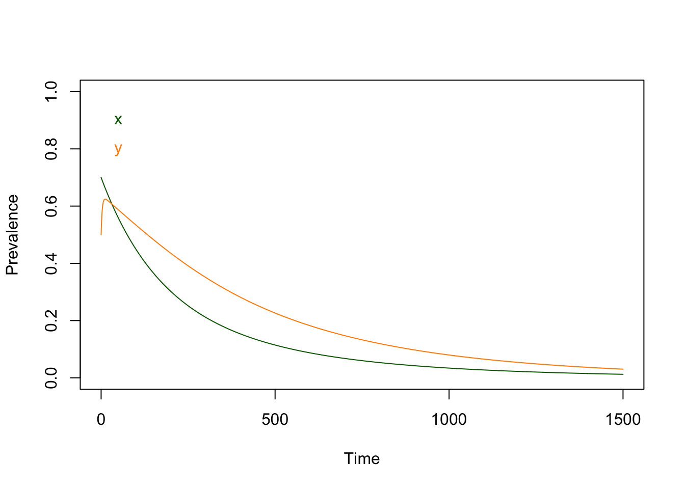
Our function ross_dts_steady_0 gives us a negative number.
ross_dts_steady_0(ross_dts_par1) x y
-0.1200000 -0.4285714 If we look at the equations, it’s easy enough to spot the problem. Since \(x\) and \(y\) must be positive, then it must be true that \[m a^2 > su.\] We call this a threshold condition.
m_crit = with(ross_dts_par, s*u/a^2)
m_crit
[1] 0.008If we check, we find that this gives us the disease free equilibrium.
ross_dts_par2 = ross_dts_makepars(m=m_crit)
ross_dts_steady_0(ross_dts_par2)
x y
0 0 It doesn’t make sense to have a negative amount of malaria. Since ross_dts_steady_0gives us negative numbers, we can use this little bit of information to write a better function, one that returns \(0\) instead of a negative number:
# INPUTS
# params - the parameters, as a list
#
# OUTPUTS
# the steady state values of x and y
ross_dts_steady_1 = function(params){with(params,{
  xx = ifelse(m*a^2 > s*u, (m*a^2 - s*u)/(m*a^2 + s*a), 0)
  yy = a*xx/(u+a*xx)
  c(x=xx,y=yy)
})}ross_dts_steady_1(ross_dts_par1)x y
0 0 In A Ross-Macdonald Model, we’ll take another look at thresholds.
A lot of analysis can be done with a pencil and paper, but this book is taking a computational approach. Here, we introduce some conventions that we will use to build software that can support robust analytics.
Computers are very good at repeating tasks, but if we want to get the computers to repeat tasks efficiently, we must write some code that is designed for that task. One useful trick is to write functions that call other functions to expedite workflows. In this case, we want to write a function that solves the equations (i.e. that iteratively computes and stores the values) over some time interval:
# INPUTS
# pars - the parameters, as a list
# x0   - the initial value of x
# y0   - the initial value of y
# t0   - the initial value of t
# tmax - the last value of t
#
# OUTPUTS
# the values of the variables over time, as a list
ross_dts_solve_1 = function(pars, x0=.01, y0 = 0.001, t0=0, tmax=100){
   xy = c(t=t0, x=x0, y=y0)
   xy_t = xy
   for(t in (t0+1):tmax){
     xy = ross_diffs_1(xy, pars)
     xy_t = rbind(xy_t, xy)
   }
   return(list(time=xy_t[,1], x=xy_t[,2], y = xy_t[,3], last = xy))
}
We can write another function that plots the equations (i.e. that iteratively computes and stores the values) over some time interval:
# INPUTS
# xy_t - a list with elements named x, y, and time
# type - plot type:  "l" or "p" or "b"
# lty  - lty
# add  - if TRUE, add to existing plot
#
# OUTPUTS
# the values of the variables over time, as a list
plot_xy = function(xy_t, type = "l", lty=1, add=FALSE){with(xy_t,{
  if(add == FALSE)
  plot(time, x, "n", ylim = range(0, 1, y, x), ylab = "Prevalence", xlab = "Time")
  lines(time, x, type = type, lty=lty, col = "darkgreen", pch =15)
  lines(time, y, type = type, lty=lty, col = "darkorange", pch =19)
  text(0, 0.9, "x", col = "darkgreen", pos=4)
  text(0, 0.8, "y", col = "darkorange", pos=4)
})}
Now, we can define, solve and plot a model in a single line of code:
plot_xy(ross_dts_solve_1(ross_dts_makepars(), tmax=40), type="p") 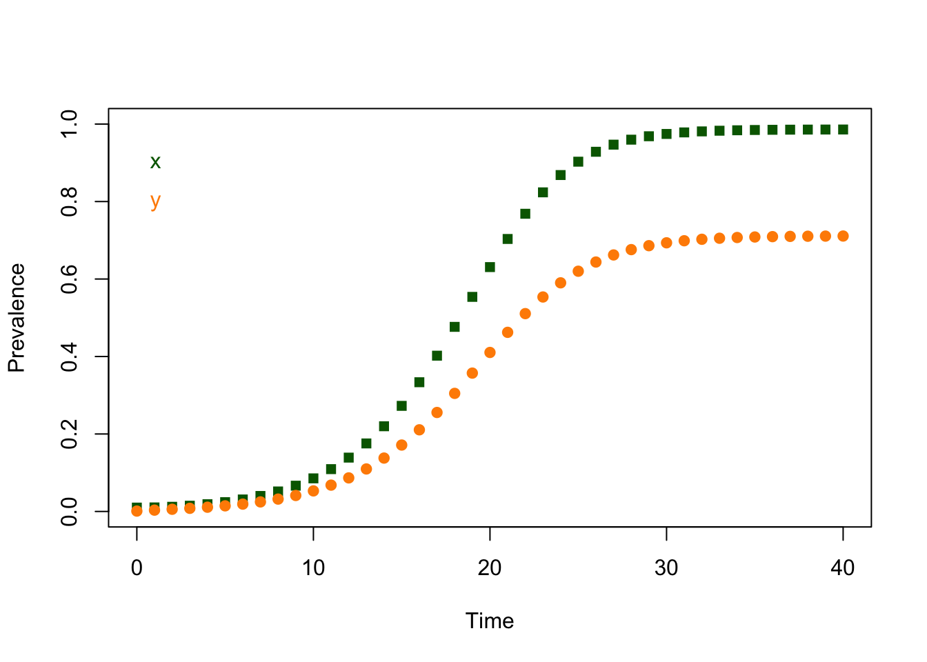
We’re not necessarily advocating that we write all code this way. The first version of code is for us, but if we want someone else to follow our code, we should make it easy to follow. It should be easy to find and diagnose problems, and it should be easy for someone else to use it. If we go to the trouble, the logic is nested in a set of function calls, and it’s easy to follow the algorithm. For example, everything we’ve done above is in these three
# Make a parameter set
params <- ross_dts_makepars()
# Solve the equations
output <- ross_dts_solve_1(params, tmax=40)
# Plot the outputs
plot_xy(output, type="p") 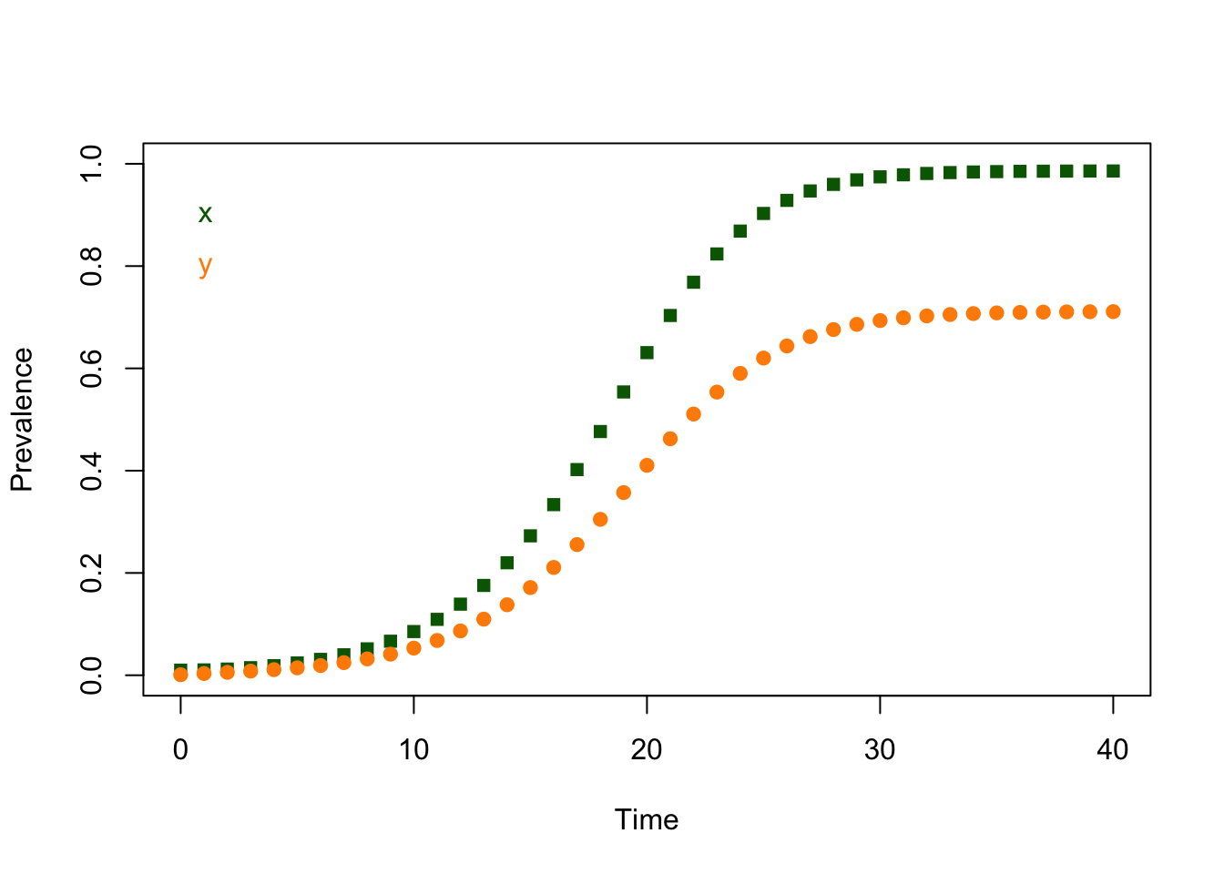
If we’re going to take ourselves seriously, we want to get used to double checking everything to avoid making and propagating mistakes. One way to do this is to find two or more ways of computing the same thing. We’re trying to check that the code does what we claim it does, a process called verification.
If we’ve done everything right, we ought to get the same values for the steady states through our analysis and simulation.
The last values of \(x\) and \(y\) from the simulation are:
output$last[-1] x y
0.9859663 0.7109837 The last values of \(x\) and \(y\) from evaluating ross_dts_steady_1() are:
ross_dts_steady_1(params) x y
0.9861386 0.7114286 It’s tempting to look at the printout and assume these two numbers are exactly equal, but when we deal with computers, everything gets computed and stored using some number of memory bytes. We can never be sure that a match will be be exact. We can simply sum up the absolute values of the differences:
sum(abs(output$last[-1] - ross_dts_steady_1(params)))[1] 0.0006171682If we wanted to reduce this to a simple error check, we should pick a tolerance level – say \(10^{-9}\) – and then just ask if we are closer than that:
# INPUTS
# xy  - xy
# par - a set of parameters for a ross_dts model
# tol - a tolerance level
#
# OUTPUTS
# boolean -
ross_dts_checkit_1 = function(params, tmax=200, tol=1e-9){
  xy1 <- ross_dts_solve_1(params, tmax=tmax)$last[-1]
  xy2 <- ross_dts_steady_1(params)
  sum(abs(xy1 - xy2)) < tol
}
There are decisions to make. How long should we run the model? If we don’t run the simulation model for long enough, it will not have converged.
ross_dts_checkit_1(ross_dts_par, tmax=40)[1] FALSEIn this case, the model converges for the default value of tmax that we set:
ross_dts_checkit_1(ross_dts_par, tmax=200)[1] TRUEThere is a problem with ross_diffs_1. If we set \(m\) too high, such that at some point \(m a y_t > 1,\) then the whole system eventually crashes:
ross_dts_par3 = ross_dts_makepars(m=12.4)
plot_xy(ross_dts_solve_1(ross_dts_par3, x0 = .01, y0=.001, tmax=50), "b") 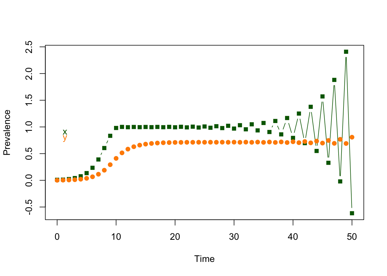
We need a good way of dealing with the problem that gave rise to this numerical instability. The question at hand is what fraction of people would become infected, on average, if the expected number of bites was \(may_t?\) Ideally, we want to return a proportion, even when \(may_t>1.\) We call this quantity – the fraction that gets infected in a day – the daily attack rate.
How should we compute the probability of infections if we expect to get exposed more than once?
In discrete time formulations, we must be very careful to ensure that we have formulated a proper model. How can we fix this problem? We have to go back and rethink the way we formulated our model. How does the probability of getting infected scale with the number of infective bites?
If we knew that there were exactly an integer number of bites, \(ma,\) then the proportion of people not getting infected would be those that didn’t get infected from any one of the bites, or \((1-y_t)^{ma}.\) There is, however, an even better way to think about this.
In a lot of cases like this, without any other information, we would assume that the number of bites, per person, would follow a Poisson distribution. It’s actually easier to say who doesn’t get infected, and that’s the zero term of a Poisson, \(e^{-may_t}.\) The probability of getting infected is the complement of the probability of getting at least one bite, or
\[1 - e^{-m a y_t}\]
Equations
Our variables, initial conditions, and parameters are all defined in the same way as ross_diffs_1, but now our equations have changed:
\[ \begin{array}{rl} x_{t+1} &= x_t - s x_t + (1-e^{-m a y_t}) (1-x_t) \\ y_{t+1} &= y_t - u y_t + a x_t (1 - y_t) \\ \end{array} \tag{4}\]
As before, we write a function to numerically solve the discrete time system:
# INPUTS
# xy      - current variables, as a named vector
# params  - the parameters, as a list
#
# OUTPUTS
# the updated values of the variables, as a named vector
ross_dts_2 = function(xy, params){with(as.list(xy), with(params,{
  xn = x - s*x + (1-exp(-m*a*y))*(1-x)
  yn = y - u*y + a*x*(1-y)
  t=t+1
  return(c(t=t, x=xn, y=yn))
}))}
Once again, we can wrap a function around the solver so that it’s easier to use the code:
# INPUTS
# pars - the parameters, as a list
# x0   - the initial value of x
# y0   - the initial value of y
# t0   - the initial value of t
# tmax - the last value of t
#
# OUTPUTS
# the values of the variables over time, as a list
ross_dts_solve_2 = function(pars, x0=.01, y0 = 0.001, t0=0, tmax=100){
   xy = c(t=t0, x=x0, y=y0)
   xy = c(t=0, x=x0, y=y0)
   xy_t = xy
   for(t in (t0+1):tmax){
     xy = ross_dts_2(xy, pars)
     xy_t = rbind(xy_t, xy)
   }
   return(list(time=xy_t[,1], x=xy_t[,2], y = xy_t[,3], last = xy))
}
Now, we can visualize the output using code we’ve already written, and can see that we have fixed our stability problem.
plot_xy(ross_dts_solve_2(ross_dts_par3, x0 = .01, y0=.001, tmax=20), "b") 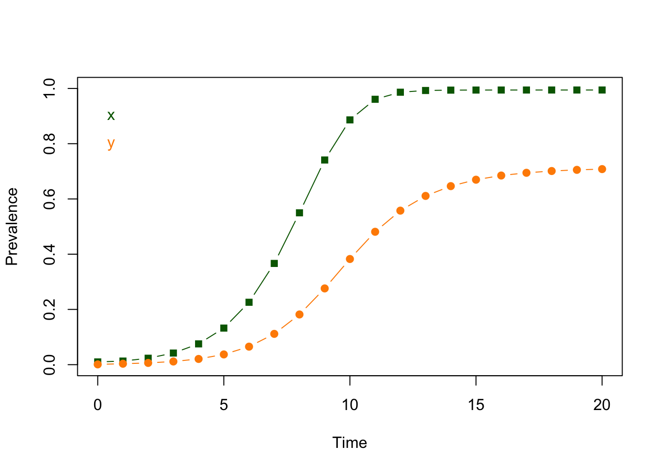
Verification
For verification, we want a method to solve things two different ways. If we want to compute the steady state, we’re stuck with the problem of solving this equation:
\[(1-e^{-m a^2 x/(u + a x)}) (1-x) = sx\]
It’s surprisingly easy to write down equations, like this one, that we can’t solve with pencil and paper. We can still find a way of computing the steady state, but we have to write R code that solves for \(x\) numerically.
# INPUTS
# par - the model parameters, as a list
#
# OUTPUTS
# the steady state values of x and y
ross_dts_steady_2 = function(pars, tol=1e-10){with(pars,{
   f_xx = function(x, pp){with(pp,{
     xx = (1 - exp(-m*a^2*x/(u+a*x)))*(1-x) - s*x
     y = a*xx/(u+a*xx)
     yy = u*y + a*xx*(1-y)
     return(xx^2 + yy^2)
   })}
   xx = optimize(f_xx, c(0,1), pp=pars, tol = tol)$min
   yy = a*xx/(u+a*xx)
   c(xx, yy)
})}
Finding the equilibrium this way, we get:
ross_dts_steady_2(ross_dts_par3)[1] 0.9944158 0.7131415Second, by getting the solution after many iterations.
ross_dts_solve_2(ross_dts_par3, x0=.1, y0=.05, tmax=300)$last[-1] x y
0.9944158 0.7131415 By inspection, these two numbers are very close, but not exactly matching. Once again, we want to ensure that our code does not have any mistakes, so we write a function to verify our results. We set a term that describes an acceptable tolerance for computational errors, and ask if we’re at least that close.
# INPUTS
# xy     - xy
# par    - a set of parameters for a ross_dts model
# tmax   - maximum runtime for ross_dts_solve_2
# st_tol - tolerance for ross_dts_steady_2
# tol    - desired tolerance for verification
#
# OUTPUTS
# boolean -
ross_dts_checkit_2 = function(params, tmax=300, st_tol=1e-10, tol=1e-7){
  xy1 <- ross_dts_solve_2(params, tmax=tmax)$last[-1]
  xy2 <- ross_dts_steady_2(params, tol=st_tol)
  sum(abs(xy1 - xy2)) < tol
}
Do the two answers differ by less than \(10^{-7}\)?
ross_dts_checkit_2(ross_dts_par3)[1] TRUEIt’s a little unsatisfying to get numerical errors, but machines don’t do exact computation easily. We’re interested in getting as close as we need to get without doing a lot of work that would, in the end, never make a difference. The operating principle here is that we need to be sure that our code is doing what we think it should, and that it is giving answers that are close enough.
Also of interest, discrete time model ross_diffs_2 was implemented in a Google Sheet.