Reproductive Numbers
An Introduction to Thresholds

The basic reproductive number, \(R_0\) is a useful way of understanding dynamical systems describing malaria. Here, we present a generalized approach to the computation of threshold criteria for heterogeneous systems.
See Related for links to closely related vignettes.
In 1952, George Macdonald presented a formula for \(R_0\) for malaria as a threshold condition for malaria persistence [1]. Here, we present a generalized approach to computing thresholds for some closed heterogeneous dynamical systems:
spatial dynamics are patch-based / metapopulation dynamics [2]
seasonality allows forcing on any of the terms.
The algorithms to compute \(R_0\) have been implemented in SimBA, a suite of R software packages designed to support simulation-based analytics for malaria and other mosquito-borne pathogens.
We understand \(R_0\) as a spectral average:
It is the asymptotic growth rate of a linearized system, evaluated at the disease-free equilibrium
It is the lead eigenvalue of the next-generation matrix.
In developing this, we rely heavily on the next-generation matrix approach developed by Diekmann et al. and also by van den Driessche and Watmough for threshold criteria for structured population models [3,4].
In developing these methods, we recognize a difference between the definition of a generation that would be used by any parasitologist or biologist, and the one used by mathematicians. We formulate a next-generation matrix for malaria parasites using formulas that generalize the concepts of vectorial capacity and the human transmitting capacity for spatially and temporally heterogeneous systems, and we show that it is equivalent to the next-generation matrix approaches that have proven so useful in mathematics.
Generically, suppose we have a dynamical system describing malaria transmission dynamics. We want to develop a metric that serves as a threshold criterion for closed systems, and that can be used to benchmark models. This is an outline:
\[M^t = \sum \lambda_i^t X_i\] # Simple Systems
\(V\) - Vectorial Capacity
\(D\) - HTC
In autonomous, 1-patch systems with no control:
\[R_0 = V D\]
Spatial Dynamics
\([V]\) - VC Matrix
\([D]\) - HTC Matrix
Next generation spatial matrices:
\([R_x] = [V]\cdot[D]\) - from human to human
\([R_z] = [D]\cdot[V]\) - from mosquito to mosquito
Thresholds:
\([R_x] \cdot \tilde X = \lambda \tilde X\) where \(\lambda\) is a scalar, then \(\tilde X\) is an eigenvector
\([R_z] \cdot \tilde Z = \lambda \tilde Z\) where \(\lambda\) is a scalar and \(\tilde Z\) is an eigenvector.
The largest \(\lambda\) is called the dominant eigenvector or the spectral average, and \(\tilde X\) or \(\tilde Z\) are the associated eigenvectors.
Connectivity
We can rewrite:
\([D] = D [K_D]\), where \(D\) is a scalar value and \([K_D]\) describes parasite dispersal among patches by humans
\([V] = V [K_V]\), where \(V\) is a scalar value and \([K_V]\) describes parasite dispersal among patches by mosquitoes
Now connectivity from any starting set of bites is
\([C_x] = [V]\cdot[D]\cdot \left< X \right>\)
\([C_z] = [D]\cdot[V]\cdot \left< Z \right>\)
The \(R_0\) versions of this are:
\(X = \tilde X\)
\(Z = \tilde Z\)
At the endemic equilibrium, \(X = fqZ\) and \(Z = \kappa\)
Forcing
When VC varies from day-to-day, we need functions to describe the temporal dispersion of a parasite generation in mosquitoes and in humans.
\(V(t)\) is the VC on day \(t.\) The number of infective bites arising at time \(t+\ell\) is \(V_\ell(t,\ell)\) such that \[V(t) = \int_t^\infty V(t ,\ell) d \ell\] and the annual average VC is: \[V_A = \int_0^{365} V(t) \; dt\]
\(D(t)\) is the HTC on day \(t.\) The infectiousness on day \(\ell\) of an infection that started on day \(t\) is: \(D_\ell(t,\ell)\) such that \[D_\ell(t) = \int_0^\infty D(t, \ell) d \ell\] and the annual average HTC is: \[D_A = \int_0^{365} D(t) \; dt\]
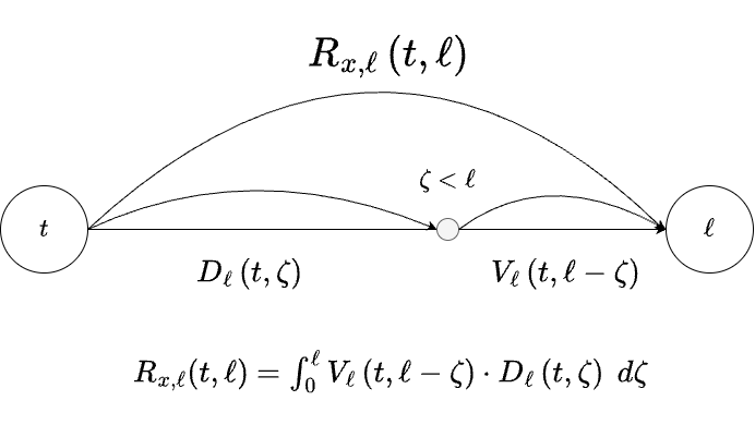
For one complete generation, we need to compute convolutions. The number of infections at lag \(\ell\) after the infection: \[R_{x,\ell}(t, \ell) = \int_0^\infty V_\ell(t, \ell-\zeta) D_\ell(t, \zeta) d\zeta\] so the number arising from infections at time \(t\) is \[R_x (t) = \int_0^\infty R_{x, \ell}(t, \ell) d \ell\] or \[R_z(t, \ell) = \int_0^\infty D_\ell(t, \ell-\zeta) V_\ell(t, \zeta) d\zeta\] and \[R_z(t) = \int_0^\infty R_{z, \ell}(t, \ell) d \ell\]
We want to deal with canonical seasonal patterns where \[V(t+365) = V(t)\]
We want to wrap offspring generated over many years in the future by time of year, so we write
\[R(d) = \sum_{d+i\; 365} R(t)\] where \(i\) is all the counting numbers.
Let the number of infections occurring on day \(d\) be \(X(d)\) and \(Z(d),\) and we compute \[R_x(t) \tilde X(d)\] and after wrapping, for all \(d\):
\[R_x(d) \tilde X(d) = \lambda R_x(d)\] or we compute \[R_z(t) \tilde Z(d)\] and after wrapping, for all \(d\):
\[R_z(d) \tilde Z(d) = \lambda R_z(d)\] then \(\tilde X\) and \(\tilde Z\) are called the temporal eigenfunctions, and the largest value of \(\lambda\) is called the spectral average.
General
Now, we put it all together:
\([V](t)\)
\([D](t)\)
The spatial-temporal next-generation matrix is:
\([R](t)\)
\([Z](t)\)