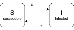
The simplest model for the dynamics of human malaria infections is called the SIS compartment model. Humans in a population are classified as being either uninfected and susceptible to infection \((S)\), or infected and infectious \((I)\). After recovering from infections, humans are susceptible.
Fig 1: A diagram of the SIS Compartment Model
The Model
Malaria is complex, but a good starting point is a simple model, called the SIS compartment model. A population is subdivided into susceptible (\(S\)) and infected and infectious (\(I\)) individuals, where the total population is \(H = S+I.\)
We let \(h\) denote the force of infection (FoI).
We let \(r\) denote the clearance rate for infections.
We assume that individuals become susceptible after recovering (See Fig. 1).
The dynamics are described by a pair of equations:
\[
\begin{array}{rl}
\dot{I} &= h S - rI \\
\dot{S} &= -hS + rI
\end{array}
\]
If we know \(H\), then one of these equations is redundant. Here, we compute:
\[
\dot{I} = h (H-I) - rI
\]
Steady States
Let the variable \(x\) denote the fraction infected, \((x = I/H)\). Substituting, we get:
\[
\dot{x} = h (1-x) - rx
\]
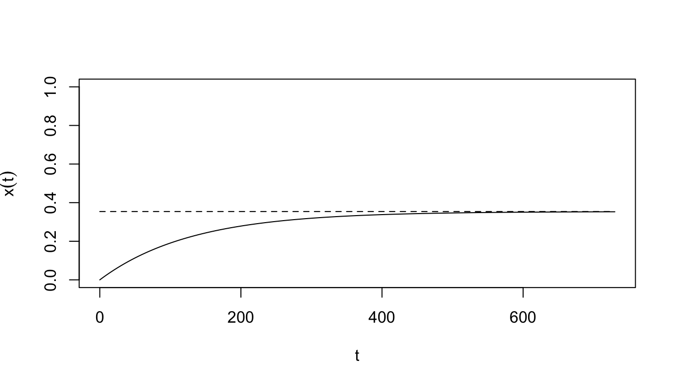
If \(h\) is constant, then we can easily compute prevalence at the steady state (denoted \(\bar x\)):
\[\bar x = \frac{h}{h+r}\]
At the steady state, the odds of infection are:
\[ \frac{\bar x}{1- \bar x} = \frac {h}{r}\]
Solutions
We can solve the equation above. Assuming no one is initially infected at time \(t=0,\) (i.e.\(x(0) = 0\)), the prevalence of infection increases dynamics with respect to age are given by the function:
For example, in a population where the FoI is one infection per year (\(h=1/365\)), and infections last around 200 days (\(r=1/200\)), we can plot the prevalence of infection over time in a cohort that was initially fully susceptible:
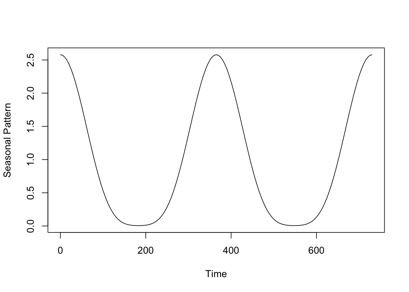
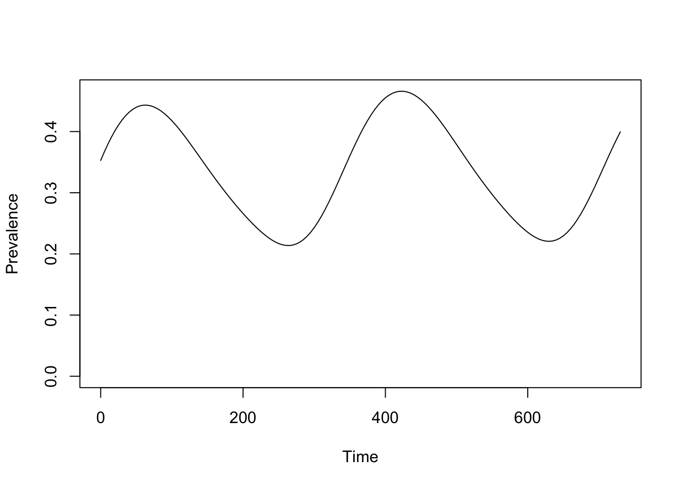
One advantage of the numerical approach is that it is not constrained by the need to find closed form solutions. For example, suppose that the FoI has a seasonal pattern:
mod <-last_to_inits(mod)mod$EIR_obj$season_par <-makepar_F_sin(bottom =0.1, pw=2)mod$EIR_obj$F_season <-make_function(mod$EIR_obj$season_par)show_season(mod)
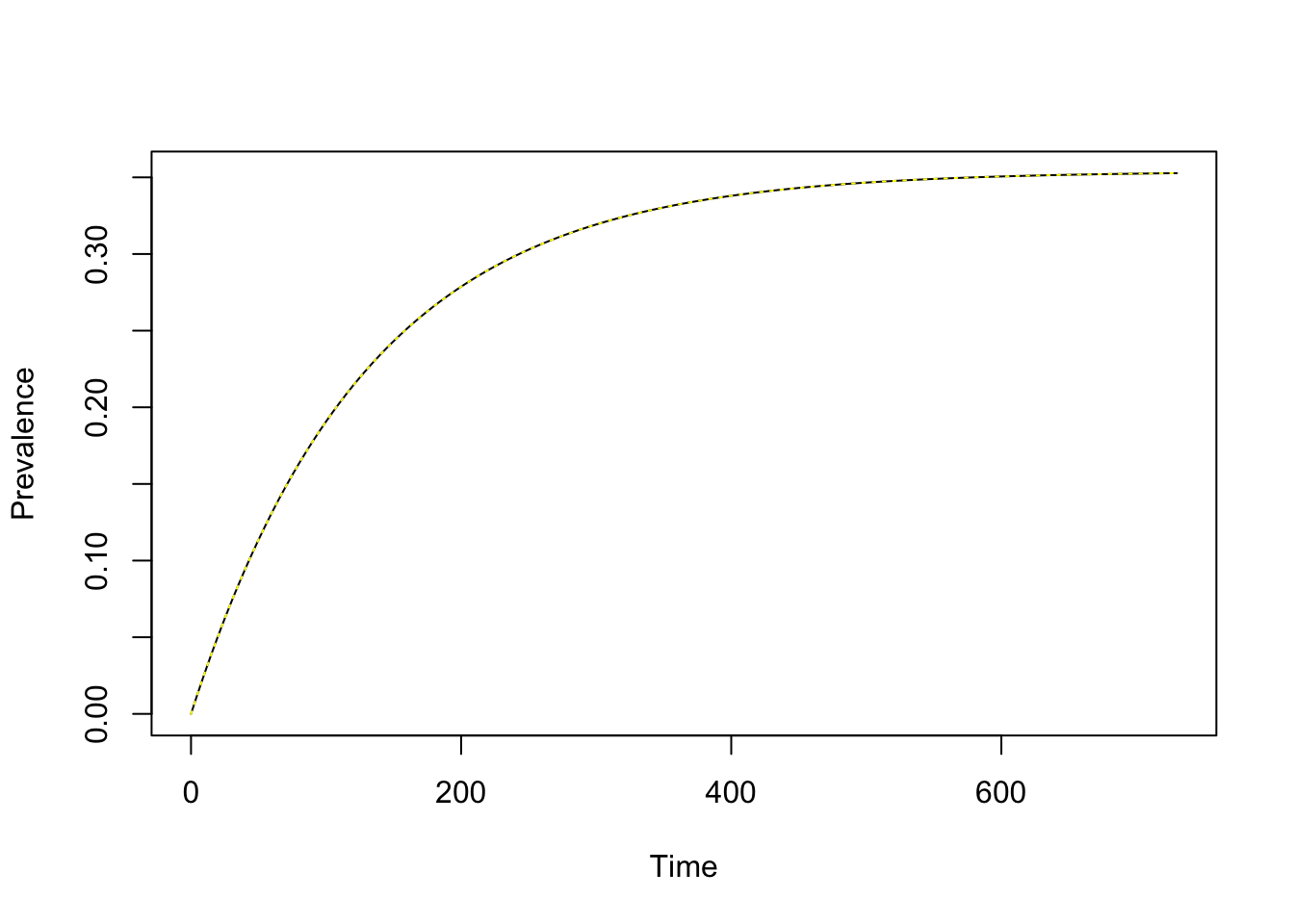
mod <-xds_solve(mod, Tmax=730, dt=5)xds_plot_PR(mod)