Chapter 15 More about data manipulations: merging, reshaping and cleaning data
In the dplyr section we discussed a large class of data manipulation operations, such as selecting variables, filtering observations, arranging data in certain order and computing new values. Here we add additional operations: reshaping.
15.1 Merging data
When working with real-world data, you’ll often find that that data is stored across multiple files or across multiple data frames. This is done for a number of reasons. For one, it can help to reduce memory usage. For example, if you have information on students enrolled in different courses, then you can store information about each course, such as the instructor’s name, meeting time, and classroom, in a separate data frame. This saves a lot of space, otherwise you have to duplicate that information for every student who takes the same course. You may also want to keep your data better organized by having student information in one file, and course information in another. This separation and organization of data is a core concern in the design of relational databases.
This section discusses how to combine such separately organized information into a single data frame.
15.1.1 Combining data frames
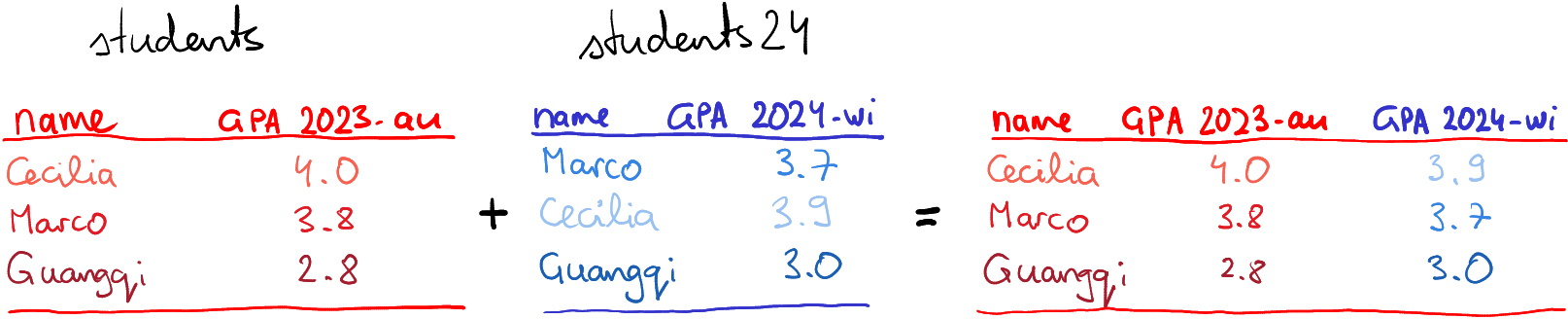
In simple cases, we may just combine datasets, row-by-row, or column by column. Consider a student dataset
students <- data.frame(
   student = c("Cecilia", "Marco", "Guangqi"),
   "GPA 2023-au" = c(4.0, 3.8, 2.8),
   check.names = FALSE)
students
## student GPA 2023-au
## 1 Cecilia 4.0
## 2 Marco 3.8
## 3 Guangqi 2.8This contains the students’ names and their GPA for 2023-au quarter.
When the following quarter ends, we may store their new GPA in a vector
## [1] 3.9 3.7 3.0Importantly, the numbers here are
in the same order as in the original data frame,
i.e. “3.9” for Cecilia and “3.0” for Guangqi.
Now we can
just “solder” this vector to the GPA data frame
using cbind() (combine column-wise):
## student GPA 2023-au GPA 2024-wi
## 1 Cecilia 4.0 3.9
## 2 Marco 3.8 3.7
## 3 Guangqi 2.8 3.0This adds another column (vector) to the data frame, and calls it “GPA 2024-wi”. gpa2024 it is just a single vector of data. But we can also combine two data frames in the similar fashion, row-by-row.
When a new student Nong arrives to the college, we can create a separate data frame for his results:
nongsGPA <- data.frame(
student = "Nong",
"GPA 2023-au" = 3.6,
check.names = FALSE) # allow non-standard name 'GPA 2023-au'
nongsGPA## student GPA 2023-au
## 1 Nong 3.6Next, we want to add it as a new row to our students’ data.
Two data frames can be combined row-wise in a fairly similar fashion
using rbind() (combine row-wise):
##   student GPA 2023-au
## 1 Cecilia         4.0
## 2   Marco         3.8
## 3 Guangqi         2.8
## 4 Nong 3.6But note the difference–now we add a row to the data frame, and a row
contains different kinds of values, in this example one of these is of
character type (“Nong”) and
one is of number type (“3.6”). Hence we need to convert the row to a data
frame, and use exactly the same column names as in the students data
frame above. rbind() ensures
that the correct columns are matched.
You can use cbind() and rbind() to combine not just single rows
and single columns but two larger data frames. This is a very simple
way of joining data frames, in the sense that each
row will be combined with the corresponding row, or each column with
the corresponding column. If the students in the 2024-wi data are in
a different order, the result will be wrong.
Below, we discuss more complex merging that ensures that even if the order differs, the results are still correct.
15.1.2 Merging by key
The simple way of combining data frames what we did above–just adding those row-wise, is fairly limited. What happens if new students join the college, or previous students leave? Or if just the data is ordered differently? In such cases we need to merge rows in two tables not by their order (row number), but we need to find the corresponding rows in both tables. This is merging by key.
15.1.2.1 Merge key
For instance, imagine that in winter 2024 the student list looks somewhat different:
students24 <- data.frame(
   student = c("Cecilia", "Guangqi", "Nong"),
   "GPA 2024-wi" = c(3.9, 3.0, 3.6),
   check.names = FALSE)
students24
## student GPA 2024-wi
## 1 Cecilia 3.9
## 2 Guangqi 3.0
## 3 Nong 3.6If we were just to use cbind() here, we’d create quite a mess:
##   student GPA 2023-au students24$`GPA 2024-wi`
## 1 Cecilia         4.0                      3.9
## 2   Marco         3.8                      3.0
## 3 Guangqi         2.8                      3.6
While all is well with Cecilia, now Guangqi’s winter quarter grades are assigned to Marco, and Guangqi in turn gets Nong’s winter grades. This will cause a lot of trouble for the university!
What we need to do instead is to find which line in the first dataset (autumn 2023) corresponds to which row in the second dataset (winter 2024), and combine those rows. This is the idea of merging or joining (because you are “merging” or “joining” the data frames together).
Before you can actually do any merging, you need to find some kind of identifiers, values that determine which row in the first data frame corresponds to which row in the second data frame. In this case it is easy–it is the students’ names. We have to ensure that Cecilia’s grades from one quarter are merged with her grades in the next quarter, and the same for Quangqi, Marco and others.
This value, or a set of values, is called merge key. We cannot do any merging before we have identified the merge key. There are multiple kinds of merge keys:
- primary key is the key in the current data frame.
- foreign key is the key in the other data frame. It may be a column with the same name, or it may also have different names across different datasets. And be aware–sometimes a column with a similar name has a different meaning in different datasets!
- Often, a single column is enough to identify the records. The example above can be merged correctly by using just name. But sometimes you need multiple columns, such as year and month. This is called compound key, a key that consists of multiple columns.
- If there is no good identifier, we may create one from what we have. This is called surrogate key. For instance, it is common to link personal datasets using name and day of birth. This usually works, but may create problems if two persons of the same name are born in the same day. Another problem with this surrogate key is the habits to write names in many slightly different forms. For instance, are “John Smith”, “John A. Smith” and “John Alexander Smith” the same person?
15.1.3 What to merge and what not to merge?
Before you even begin with merging, you should ask if these datasets can be merged? And even if you can merge these, does it make sense? Do you want these to be merged? We discuss here a few examples.
Students:
| name | course | quarter | year |
|---|---|---|---|
| Ernst | info201 | 2023-au | 1 |
| Ernst | math126 | 2023-au | 1 |
| Ernst | cse120 | 2024-wi | 1 |
| Eberhard | arch101 | 2023-au | 2 |
| Eberhard | info201 | 2024-wi | 2 |
| … | … | … | … |
Courses:
| name | quarter | day | time | instructor |
|---|---|---|---|---|
| info201 | 2023-au | Tue | 10:30 | Schnellenberg |
| info201 | 2024-wi | Tue | 10:30 | Schnellenberg |
| math126 | 2023-au | Thu | 1:30 | Recke |
| arch101 | 2023-au | Wed | 3:30 | Plater |
| … | … | … | … | … |
Example students’ and courses’ data.
Imagine you are working at a college and you have access to students’ data (name, day of birth, address, courses they have taken, grades, and so on). You also have access to the college’s course catalog, including course number, quarter, instructor’s name, etc. Can you merge these two datasets? What might be the merge key? Why may you want to do that, what interesting questions can be answered in this way?
These two data frames can easily be merged. The key might be the course number. But should they key contain the quarter? The answer is “maybe”, depending on what kind of questions are we asking.
- If we ignore the quarter, then we merge a course called “info201” with all students who have taken “info201”. This might be useful to compare that course with other similar courses, to analyze the average grades, which other courses the students tend to take, and other course-specific questions.
- If we include quarter in the merge key, then we can answer questions about a particular course instance. For instance, we can compare different instructors of the same course, or analyze at which year students tend to take info201.
- Note that we can use one of the columns with common name, quarter, as the merge key, but we cannot use the other name, as the key. This is because in these two different tables name means different things: it is the student’s name in the first table and the course name in the second table.
All these examples are valid question that the college might want to analyze.
Exercise 15.1 Assume we merge students with courses using just course number and ignoring everything else. Provide additional examples of questions that one might want to answer with the resulting data.
| date | temp | precip | sunrise |
|---|---|---|---|
| 2024-02-21 | 9 | 0.5 | 7:03 |
| 2024-02-22 | 12 | 0.0 | 7:01 |
| 2024-02-23 | 12 | 0.0 | 6:59 |
| 2024-02-24 | 5 | 1.0 | 6:57 |
Example weather data
But imagine now that we have also weather data: for every day, we know temperature, precipitation, wind speed, and also sunrise/sunset time. Can we combine students and weather in a meaningful way? What kind of questions might we answer with such a combination?
- First, weather is not something that college can do much about. The schedules are typically planned months in advance, and it is hard to change much based on the last minute weather forecast. This means weather data is perhaps not that relevant for colleges.
- Second, what kind of meaningful questions can we answer if we have such combined data? The only questions that come to my mind is to see if there is any relationship between temperature and grades, or more likely, between sunlight hours, what time of day the course is offered, and students’ performance.
- Third, what might be the merge key? There are no course numbers nor student names in the weather table. The only possible key is date. Neither student data nor course data contains date–but course data includes quarter. So now we can compute average weather or time of sunset for the quarters from the weather data, merge this with course data, and finally combine with students’ data. This sounds complicated, but it is perfectly doable.
These examples are also valid questions, but probably ones that the colleges consider less important.
Exercise 15.2 Many common datasets contain geographic information (geolocation). Imagine you have the students data from above, but now including the geolocation of the college.
- What other kind of data you might merge with these, and what interesting questions might it answer?
TBD: complete this exercise
15.1.4 Different ways to merge data
When merging data, the computer will always find the common key values in both data frames, and merge the corresponding rows. But as usually, the devil is in the details. What should the computer do if there is not match for some of the keys in one of the data frames? Or if a key in one table corresponds to multiple lines in the other table? This is where one has to decide what is a good way to proceed.
15.1.4.1 Basic merging
Consider the student data example again. The university collects
students’ GPA information, and stores it in different data frames. In
this case these are students for 2023-au GPA, and students24 for
2024-wi GPA. However, the data frames are now ordered in an arbitrary
way:
students <- data.frame(
   name = c("Cecilia", "Marco", "Guangqi"),
   "GPA 2023-au" = c(4.0, 3.8, 2.8),
   check.names = FALSE)
students24 <- data.frame(
   name = c("Marco", "Cecilia", "Guangqi"),
   "gpa 2024-wi" = c(3.7, 3.9, 3.0),
   check.names = FALSE)
students
## name GPA 2023-au
## 1 Cecilia 4.0
## 2 Marco 3.8
## 3 Guangqi 2.8## name gpa 2024-wi
## 1 Marco 3.7
## 2 Cecilia 3.9
## 3 Guangqi 3.0cbind(). We need to ensure that the rows that
describe the same student are matched, so the first row of students
must be merged with second row of students24 and so on.
As individual students are described by name here, this columns
should be chosen as the merge key.
The following figure describes the process and the expected result:
How basic merging works: the rows of the first table are combined with
rows from the second table that match the merge key, here name.
The R syntax for merging is straightforward. For the students’ example, you can do
##      name GPA 2023-au gpa 2024-wi
## 1 Cecilia         4.0         3.9
## 2 Guangqi         2.8         3.0
## 3   Marco         3.8         3.7
More specifically, it is
where x and y are the two data frames to be merged, and key is
the names of the key columns (you need to specify it like c("name", "year") if the key contains multiple columns).
Exercise 15.3 As we discussed above, cbind() merges datasets row-by-row. So if
you merge students and students24, you’ll get Cecilia’s and
Marco’s grades messed up. Try this. What other difference can you
spot? Can you explain this behavior?
The solution
15.1.4.2 If keys do not match
But what will happen if one data frame contains keys that are not present in the other data frame?
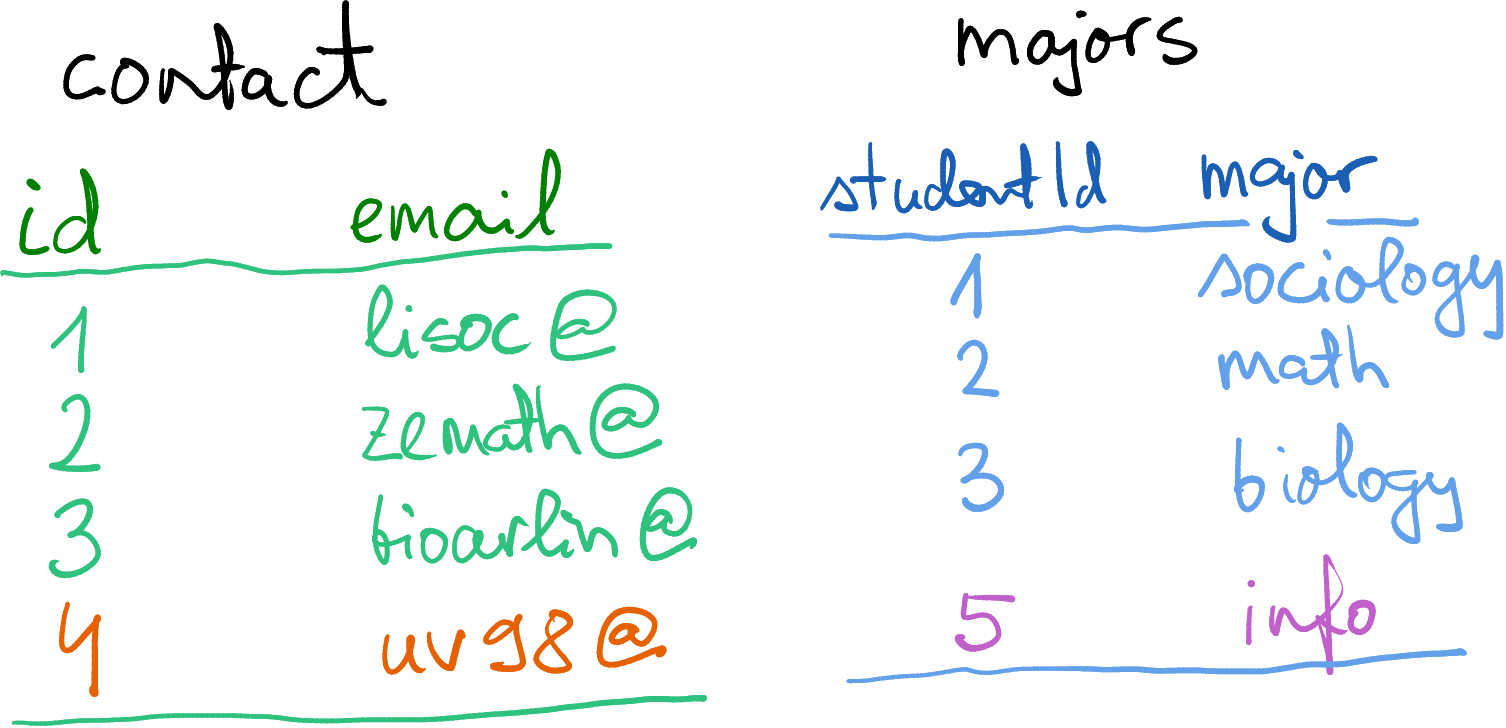
Student contact info and majors. The email domain
@college.edu is not shown.
Below, we discuss a such details using another example. Imagine you are a data scientist at a college, and you have two tables: majors for student majors, and contact for student contact information. Both of these tables use column id, the university-wide student id. (You may also have a third table that links the id to their real name, but let’s keep the names away for privacy reasons 🙂)
Importantly, as you see the student #4 does not have a major, and we do not have contact for student #5. How would you now merge these two datasets?
You may also notice that student id is denoted differently–in the
contact dataset, it is called “id” and in the majors dataset it is
“studentId”. So we need to tell merge() that the key differs
between the data frames. This can be achieved with by.x= and
by.y= as
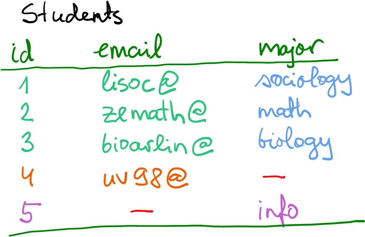
Fully merging Contact and Major by including all missing values.
Missings are here denoted by a red dash, not by NA.
But what to do with the fact that we do not know major for student #4
and email of student #5?
Obviously, you cannot fill in data you do not know, so one option is
just to use NA to mark those missing values, as shown on the figure
here.
But let’s pause before jumping into it. What do you want to do with missing majors? What do you want to do with missing emails? Why are these missing in the first place? There are different ways to proceed, depending what exactly you are doing.
First, maybe you just want to compile a comprehensive dataset of all
students. Student #4 hasn’t declared their major yet, and the email
of #5 is … just missing for some reason. Now it makes sense to
combine all data, and leave missing values as NA (or mark in another
way if you prefer). You’ll end up with a dataset that is potentially
larger (here 5 cases instead of 4), and will potentially contain
missing values.
Let’s do this on computer. First, the datasets:
contact <- data.frame(
   id = c(1, 2, 3, 4),  # student id-s
   email = c("lisoc@college.edu", "zemath@college.edu",
             "bioarlin@college.edu", "uv98@college.edu")
)
contact
## id email
## 1 1 lisoc@college.edu
## 2 2 zemath@college.edu
## 3 3 bioarlin@college.edu
## 4 4 uv98@college.edumajors <- data.frame(
studentId = c(1, 2, 3, 5), # student id-s
major = c("sociology", "math", "biology", "info")
)
majors## studentId major
## 1 1 sociology
## 2 2 math
## 3 3 biology
## 4 5 infoUsing merge() this can be done by specifying the argument
all = TRUE:
##   id                email     major
## 1  1    lisoc@college.edu sociology
## 2  2   zemath@college.edu      math
## 3  3 bioarlin@college.edu   biology
## 4  4     uv98@college.edu      <NA>
## 5  5                 <NA>      info
But in other cases you may not want to include students with missing
data. For instance, if the contact dataset is not about all
students at the college but instead a list of participants of the
student badminton club, and you are just interested to know what
majors are more common in the club. Do you really want to include
all students of the college, potentially tens of thousands, with
missing email? Obviously not. You want to preserve only those
students who are included in the contact list! In the example here,
you do not want to keep the student #5 in the final dataset. This
can be achieved by specifying all.x = TRUE, telling merge() to
include all observations from the first data frame, but only those
that have a match from the second data frame:
##   id                email     major
## 1  1    lisoc@college.edu sociology
## 2  2   zemath@college.edu      math
## 3  3 bioarlin@college.edu   biology
## 4  4     uv98@college.edu      <NA>
In other words, you want to keep all of the rows from the first table, with all of the columns from both tables. Such situations are fairly common in practice, where you want to get additional information about a small number of interesting cases from a table that contains many more cases, most of which are not interesting.
But it is not always that you want to preserve all rows of the first data frame and drop the “orphans” from the second one–sometimes want to do something else. It all depends on what kind of data do you have, and what exactly do you want to achieve.
- left join keeps all rows from the first (left) table (
all.x = TRUE) - right join keeps all rows from the second (right) table (
all.y = TRUE) - outer join keeps all rows from both tables (
all = TRUE) - inner join keeps only those rows where they keys match
Exercise 15.4
Two datasets where the column names do not match.
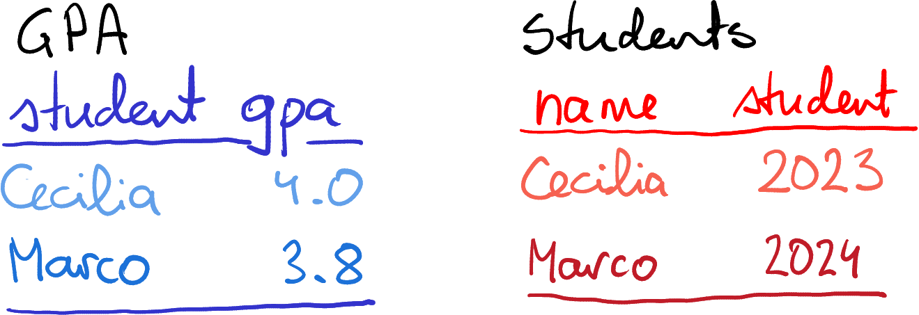
What happens if the key column names do not match? Consider two tables: GPA and Students. In the former, the column student is the student name; in the latter the name column is called name, student however is the year of enrollment.
You want to merge both tables, so the final version should include name, GPA and the year of enrollment.
- How can you tell
merge()that the key is called “student” in the first table and “name” in the second table? Hint: check out the documentation. - But both tables contain the column “student” (although they mean different things). What happens in the combined table? Does it contain two columns called “student”? Will one student-column be dropped? Something else?
- You can also merge these two tables as
merge(gpa, students). What will be the result? Can you explain why this happens?
The solution
Exercise 15.5
Consider the following tasks. Do you want to keep all cases from the first table? From the second table? From both? From neither?- You are working with mobile telephone data. You have two tables: calls that contain information about the cellphone tower where the call occurred, and towers, that contain the geographic location of the towers. You want to know where did certain calls of interest take place.
- You are working with the same telephone data. Your task is to figure out how many calls took place in one region versus another region.
- You are using a similar students’ data as in the examples above. You want to make a mailing list for all math majors.
The solution
15.1.4.3 One-to-many merge
In the previous examples, we merged tables row-by-row: one row in the original tables resulted in a single row in the final table. But that does not have to be the case. Actually, it is very common for a single row in source data to “multiply” into many rows in the final data.
Bands and songs, as separate data frames.
Consider two tables–one describes bands, the other songs. These tables can be merged using the band name, conveniently called “band” in both tables. You can see that while each band occupies only a single line in the “Bands” table, each band has multiple songs in the second table. So if we want to combine these tables–add band name, genre, and maybe the bands location to each song–then each band’s data must be present several times.
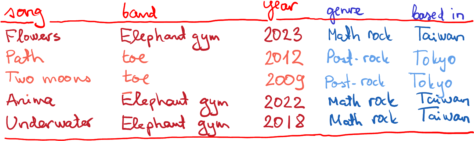
As you can see, the bands’ data has been replicated multiple times, once for each of their songs.
In terms of R syntax, there is nothing special you have to do.
merge() will take care of everything. You can just issue
While this is fairly innocent in this example, such data replication may not be a good idea in case of large datasets. If the bands dataset would contain a lot more information, including maybe their images or even videos, the result may be un-necessarily large. This is one of the reasons that large complex datasets are often kept as a set of separate tables. You can always combine those if needed, but maybe you want first to select the relevant cases only, before you merge the rest.
Exercise 15.6
Customers:
| id | name | age |
|---|---|---|
| 101 | Jay | 20 |
| 102 | Bhagavad | 30 |
| 103 | Arjuna | 40 |
| 104 | Tara | 50 |
Orders:
| id | customer | amount |
|---|---|---|
| 1001 | 101 | 25 |
| 1002 | 103 | 52 |
| 1003 | 103 | 120 |
| 1004 | 103 | 170 |
| 1005 | 101 | 70 |
| 1006 | 102 | 75 |
| 1007 | 107 | 140 |
Customers and orders data tables.
You are a data scientist at a retail firm. You have two tables, one that keeps the customer data, and another one that contains data about the 2024 orders. Here is the code you can use to create the tables
- Who is the most valuable customer overall (i.e. spent most money through the year).
- Why is the most valuable young customer (i.e. below age 35).
- What was the total amount spent by Bhagavad?
- What is the merge key? Does it differ between the tables?
- How would you merge these tables? Do you want to keep all customers? Do you want to keep all orders? Does it differ from question-to-question?
- How many rows would the combined table contain if you only keep those rows where the key matches?
- Merge the data frames and answer your boss’s questions!
The solution
15.1.4.4 Many-to-many merge
It is also possible to merge data in the way that everything in one data frame will be merge to everything in the second data frame. Here is a small example:
##   a b
## 1 1 a
## 2 2 a
## 3 1 b
## 4 2 b
As you can see, the first row of df1 is replicated twice, once for
each row of df2. And the same is true for every row for both data
frames. Technically, such way of joining data frames is called
cross-join or Cartesian join.
Why does such everyone-to-everyone merge happens here? This is
because there is not merge key. Obviously, we can discuss whether the
data frames can even be merged if there is not key–but merge()
takes a view that everything can be merged with everything. (This can
also be achieved by specifying the merge key by = NULL.)
Now, when you see how such merge can be done from the technical perspective, you may be puzzled about why on earth does anybody want to do that. Why should someone want to basically copy one data frame at the end of the other many times? In fact, Cartesian join is quite useful if you are looking to get all combinations of two variables. Imagine that you are working for a large whole-sale company, who is analyzing the daily orders of all your customers. You may have a table of all your business days, and another table of all your major customers:
businessdays <- data.frame(
   date = c("2025-11-10", "2025-11-12", "2025-11-13"))
customers <- data.frame(
   customer = c("Amazon", "Booking.com", "Baidu"))
merge(businessdays, customers)
## date customer
## 1 2025-11-10 Amazon
## 2 2025-11-12 Amazon
## 3 2025-11-13 Amazon
## 4 2025-11-10 Booking.com
## 5 2025-11-12 Booking.com
## 6 2025-11-13 Booking.com
## 7 2025-11-10 Baidu
## 8 2025-11-12 Baidu
## 9 2025-11-13 BaiduNow you may to add a column sales that is initially set to 0, and later replace the zeros with the actual sales figures.
Here are a few examples:- You want to make special “menu” offers of starter and main dish in a restaurant. You combine all selected starters with all selected mains. As a baseline, the price of the menu will be the same as sum of the two dishes. But now you can replace certain baseline prices with special “combo prices”.
- You want to order shirts of different size and color for an outfit store. For your order, you combine all sizes with all available colors, and then fill in the actual order numbers for each combination.
Exercise 15.7 Give a few more examples of where cross-join might be useful!
Exercise 15.8 You have two data frames, df1 of dimensions \(40\times17\) and df2 of dimension \(100\times20\). What is the dimension of the result if you cross-join these two data frames?
Exercise 15.9 You want to create a \(5\times5\) grid as a data frame. You have
vectors x <- seq(0, 1, length.out = 5) and y <- seq(0, 1, length.out = 5).
- Use
merge()to create a data frame with two columns, x and y, so that there is a row for each combination of x and y.
15.1.5 Joins and pipes
The merge() function, as any other R function,
supports feeding data in through pipes, and sometimes it is eactly
what you may want to do. But piping data to merge may not be the best
option.
Pipe is an excellent tool if your function takes in a central, most
important argument, for instance a dataset, and returns the same
dataset that is modified in a certain way. This applies to all dplyr
functions, such as filter() or mutate(). Forwarding such central
argument allows you
to write long pipelines–each function in the pipeline modifies the
dataset and forwards it to the next function.
merge() however, is different–it takes two central inputs. It
makes a single dataset out of two datasets, and hence such pipelines
may not be possible. It is possible though to write a pipeline along
the lines
Here we work with data1, and later merge it with data2. But whatever pre-processing you do with data2 cannot be included in the same pipeline. Although it may be possible to design such merging pipelines, it is probably not worth the effort, as they lose the main reason for pipes–the intuitive order of tasks.
15.2 Reshaping data
Above, in Section 12, we discussed how many types of data can be stored in data frames, rectangular tables of rows and columns. But it turns out that the exact same information can be stored in multiple ways. Here we discuss two of the most popular forms, long form and wide form, and reshaping–the process of transforming the one to the other.
15.2.1 Motivating example
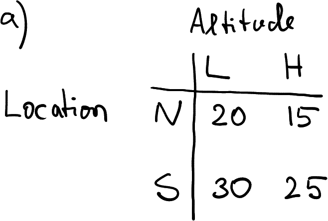
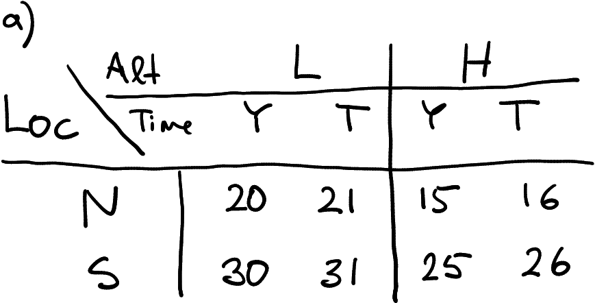
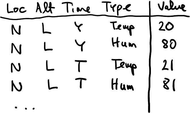
Temperature data, collected in two locations (N and S) at two altitudes (L and H).
Imagine you are a researcher at a meteorology institute. Every day you collect air temperature data at two locations: North (N) and South (S), and at two altitudes: Low (L) and High (H). An example of the data you just collected may look like in the table at right, here temperature in North at low altitude was 20, and in South at high altitude was 25.
How you might represent these data? The table at right offers one example. It is a rectangular table (data frame) that contains two rows, one for each location, and two columns, one for each altitude.
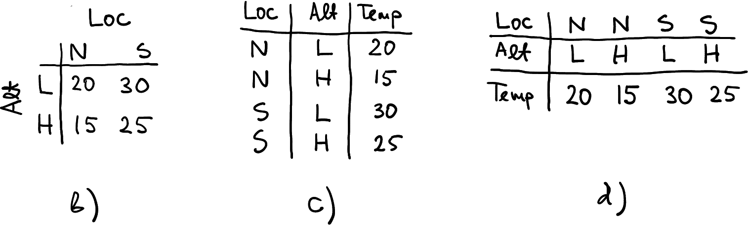
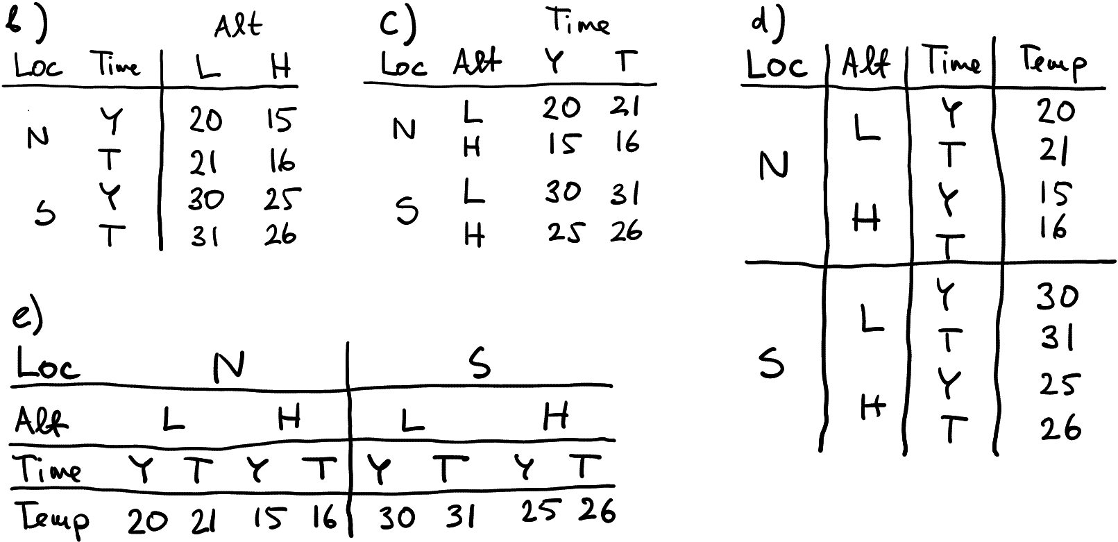
Three other ways to represent the same data
The first of these three examples, b), is just a transposition of the original table a). The other two c) and d), are “made of” the original table, but not by simple operations like transposition. You may notice though that c) and d) are basically transpositions of each other. But in any case, data in these tables is the same. All four agree that temperature in South at low altitude was 30, and the same for North-high was 15. It is not that some tables are correct while others are wrong. They are all correct. Let’s now discuss in which sense do these tables differ.
The original table a) has location in rows and altitude in columns. So here a row represents a location, and each column is an altitude, corresponding to that location. If you want, different altitude values are grouped together into the corresponding locations. The table b) is similar in many ways. But instead of grouping altitudes together into rows representing locations, it groups locations together into rows representing altitudes.
Finally, tables c) and d) discard any groupings and just put all the measures underneath each other (c) or next to each other (d). Obviously, now each row or column needs to have a label, telling which location and altitude the measure is taken of. This is achieved here through two additional columns (c) or rows (d).
While all these tables are correct, they are not always good for all purposes. Typically, a) and b) are better for human reading–this is because we can quickly move the eyes both left-and-right and up-and-down, and in this way compare both locations and altitude. Table c) tends to be the best for computers, but it is not always so. We’ll discuss it more below. Table d) is usually hard to use and can rarely be seen.
Are there any other options that were not represented here? Not really. Obviously, we can put S in the first place instead of N in tables a) and b), or alternatively, we can combine Loc and Alt values into a single LocAlt that might obtain values like “NH” or “S.L”. But otherwise, these four tables are all we can do.
Tables a) and b) are typically called data in wide form, and c) is called long form. To be more precise, we might call d) the wide form, and a) and b) as “middle form”. However, the words “wide” and “long” usually refer to another alternative, and as d) is rarely used, there is no need to talk about the middle forms.
Here is a little more about what is the wide form and what is the long form:
- In order to be able to talk about wide/long form, the data must have some kind of groupings. Here we have two such groupings: location and altitude. We can group values together by a similar location, or by a similar altitude.
- Besides of groups, we also need some kind of value (measure). Here it is temperature. Values are typically the most valuable part of a dataset. Indeed, the institute does not have to hire a data scientist to tell them that there exist such things like high altitude in North.
- In the long form, each row represents a single observation. Groups are not collected into the same row in any way. But we need additional columns that denote the group, in the example (table c) we need columns location and altitude. Otherwise we cannot tell which value belongs to which group.
- In the wide form, at least one group is collected into a single line. In table (a) it is location, in table (b) it is altitude. Table (d) shows an example where both groups are collected into a single line. Now we need either extra rows to tell where the groups belong to, or (more commonly), encode this information in the column names.
- It is not always clear what are groupings, what are values. It is somewhat fuzzy and depends on what you want to do.
The story gets more complicated if there are more groupings and more measures.
15.2.2 A look at data
Now it is time to look at real data. Let’s take the 2015 subset of the alcohol disorders data:
disorders <- read_delim("data/alcohol-disorders.csv") %>%
   filter(Year == 2015) %>%
   select(country, disordersM, disordersF)
disorders
## # A tibble: 5 × 3
## country disordersM disordersF
## <chr> <dbl> <dbl>
## 1 Argentina 3.07 1.17
## 2 Kenya 0.747 0.654
## 3 Taiwan 0.891 0.261
## 4 Ukraine 3.90 1.43
## 5 United States 2.93 1.73The columns disordersM and disordersF refer to the percentage of male and female population with alcohol disorders.
Which table from Section 15.2.1 this printout corresponds to? Is it (a), (b), (c), or (d)? It is fairly easy to see, that it is basically the same as table (a) (or b): instead of two locations, each row represent five countries. And instead of two altitudes, the columns represent two sexes.
You can also see that the data has two grouping dimensions: country and gender. The data is grouped into countries, so each row corresponds to a country, and each column (except country) is a measure of alcohol disorders. The column names also carry important information, they tell which gender the particular numbers correspond to. And finally, all the cells contain a similar measure: percentage of population with alcohol disorders. These data are in wide form.
This form of data is very popular for a few reasons:
- It is well suited for quick visual comparison. For instance, one can easily compare males in Kenya (0.747) to males in Taiwan (0.891) and find that these values are fairly similar. We can also easily compare men and women in Taiwan (0.891 and 0.261), these figures are rather different.
- It is easy to extract individual vectors. For instance, if you want to plot alcohol usage for men versus women across the countries, then this form of data is very well suited for the task.
But the table above is not convenient for other common tasks. For instance, to find the sex and country of the largest value of alcohol disorders, one needs to either compare both disorder columns manually, or maybe write a loop over the columns instead. This can be tricky. But this kind of tasks are very common when doing data processing.
Instead, we may want to present the data in the long form, as in table c):
## # A tibble: 10 × 3
## country sex disorders
## <chr> <chr> <dbl>
## 1 Argentina M 3.07
## 2 Argentina F 1.17
## 3 Kenya M 0.747
## 4 Kenya F 0.654
## 5 Taiwan M 0.891
## 6 Taiwan F 0.261
## 7 Ukraine M 3.90
## 8 Ukraine F 1.43
## 9 United States M 2.93
## 10 United States F 1.73Here the values are not grouped in any way, all the groups (years and countries) are spread to separate rows. Also, no row contains multiple instances of the same type of value–here it means no row contains multiple disorder values. We also need one or more distinct columns to mark the group membership–a column for year, and a column for country. So the long-form data requires three columns: year, country and disorder. This is how the table above was constructed.
Now finding the maximum value is fairly easy: just find the largest value of column disorders and report the corresponding row. But unfortunately, comparing males in Kenya to males in Taiwan is somewhat more complicated–first we need to find the group of rows for Kenya, and then the male row in the Kenya group. This is not as easy as with wide form data, at least on visually.
But as we explained above, these two are just different forms of the same data, they are not different datasets. Whichever form we use, Kenyan males still have somewhat lower propensity of alcohol disorders than Taiwanese men (0.747 versus 0.891). These are the same data.
Let’s look at the difference between the wide form and long form table again. In the wide form above, each line represents a country, and each country contains a group of values: disorders for men and for women. So data is grouped in lines by country. In the long form, there is no such grouping, each line represents a country-sex combination. You can also see that in the long form, each column contains different kind of values: the first column is country, the second column is sex, and the third one is the disorder percentage. This was not the case with the wide form, in that table two columns contained the disorder percentage.
Exercise 15.10 Can you sketch an alternative way to present these data in wide form?
Exercise 15.11 How might the pure wide form data look like, where neither countries nor sexes are in different rows?
See the solution
Example 15.1 Some kind of groups are needed to make the distinction between wide and long form meaningful. But what constitutes a group may be a bit unclear. For instance, look at the height-weight data. This represents a few health-related characteristics of five teenagers:
| sex | age | height | weight |
|---|---|---|---|
| Female | 16 | 173 | 58.5 |
| Female | 17 | 165 | 56.7 |
| Male | 17 | 170 | 61.2 |
| Male | 16 | 163 | 54.4 |
| Male | 18 | 170 | 63.5 |
Is this dataset in long form or in wide form? In order to answer this question, we need to understand three things: 1) what do the rows represent; 2) what are the values–the actual data values in the table (in one or in multiple columns), and 3) what are the group indicators (in column names or in dedicated columns). The answers are:
- A row represents a person (this can be inferred, but also learned from the documentation).
- We can immediately see that each column represents a value. age, height and weight are, obviously, values. Here sex is a value too: it is not a group, but the sex of that particular person.
- Finally, we do not have any group indicators! This data is not grouped in any way, it is individual data, and hence we do not have group indicators.
Why is sex a value, not a group? This is because this dataset is about five teenagers. True, it might be about two groups, boys and girls, with three kids measured in each group (the third girl would have NA-s in every column). In that case sex would be a group indicator. This was not how the dataset was constructed though.
why aren’t age, _height and weight (or maybe even sex,age, _height and weight) just different measures for the same group (one person is one group)? You can imagine reshaping this dataframe into two columns: measure (this will be either “sex”, “age”, “height” or “weight”) and value (this would be e.g. “Female”, “16”, “173” and so on).
This is not wrong (except you cannot mix numeric and character values in the single column) but it is hardly ever useful. True, these are all measures, but there are few tasks where you may want to do similar operations with all these values. It does not make sense to put height and weight on the same plot, and filtering like
filter(value > 100)is fairly meaningless.
So it makes sense to say that these data do not have any groupings, but four different kind of values instead.
How might the wide form of these data look like? Remember: wide form has all values for the group in the same row. But here we have only trivial groups–every person forms their own group and hence the data is also in a wide form! Distinction between wide and long form is meaningful only if the data contains some kind of groupings.
Exercise 15.12 Can you envision a dataset where sex is a grouping? What role should the sex play in that case?
Exercise 15.13 Consider the following dataset: the numbers are visits at a hospital by different kinds of patients:
| pregnant | male | female |
|---|---|---|
| yes | NA | 11 |
| no | 25 | 20 |
- Is this data frame in a wide form or long form?
- Can you reshape it to the other form?
See the solution
15.2.3 pivot_longer() and pivot_wider(): reshaping between wide and long form
Fortunately, it is straightforward to convert between the wide and
long form. This is called reshaping.
The tidyr package (part of tidyverse) offers two
functions: pivot_longer() and pivot_wider(). Let’s first convert
the original disorder data frame
to the long form using pivot_longer().
For the reminder, here is the disorder data again:
| country | disordersM | disordersF |
|---|---|---|
| Argentina | 3.0698864 | 1.1703126 |
| Kenya | 0.7469638 | 0.6539660 |
| Taiwan | 0.8912813 | 0.2611961 |
| Ukraine | 3.8954954 | 1.4253794 |
| United States | 2.9275393 | 1.7291682 |
pivot_longer() takes a
number of arguments, the most important of which are cols, values_to
and names_to.
coltells which columns are to be transformed to long format. We want to transform the value columns, disordersM and disordersF. These columns contain a similar value–percentage of alcohol disorders. We do not want to convert country: this is the grouping dimension, the name of the country, not percentage of disorders (remember, these data are grouped by country and sex). The value forcolcan be specified in a similar fashion as forselect(), see Section 13.3.1. Here we can pick e.g.col = c(disordersM, disordersF)or equivalently,col = !country.values_tois just the name to the resulting value column: the two columns we selected, disordersM and disordersF will be stacked together into a single column (or more precisely, interleaved into a single column). If not specified, it will be called “value”.names_tois the name for the new grouping indicator. As disordersM and disordersF are combined together, we need a new column that tells which rows is originating from which of these. If not specified, the column will be called just “name”.
Now we are ready to do the actual reshaping. We need to select all columns except country. Lets call the resulting values “disorders”, and the other grouping column, the one that will contain the original column names “sex”:
longDisorders <- disorders %>%
pivot_longer(!country,
values_to = "disorders",
names_to = "sex")
longDisorders## # A tibble: 10 × 3
## country sex disorders
## <chr> <chr> <dbl>
## 1 Argentina disordersM 3.07
## 2 Argentina disordersF 1.17
## 3 Kenya disordersM 0.747
## 4 Kenya disordersF 0.654
## 5 Taiwan disordersM 0.891
## 6 Taiwan disordersF 0.261
## 7 Ukraine disordersM 3.90
## 8 Ukraine disordersF 1.43
## 9 United States disordersM 2.93
## 10 United States disordersF 1.73And here we have it. The long form contains three columns–two of these, country and sex are grouping indicators, and the third one disorders, contains the actual values. Note that you may want to do a bit of post-processing and remove “disorders” from the sex column leaving only “F” or “M”. It happens frequently that the column names do not make nice group indicators.
Long form is good for various kinds of data processing tasks,
but sometimes
we want to transform it back to wide form. This can be done with
pivot_wider(). The most important arguments it takes are
names_from and values_from. The former tells which column
contains the new column names–it should be one of the grouping
dimensions, here sex or country. values_from tells which column
contains the corresponding values, here it must be disorders.
So let’s get our wide form disorders
back:
## # A tibble: 5 × 3
##   country       disordersM disordersF
##   <chr>              <dbl>      <dbl>
## 1 Argentina          3.07       1.17
## 2 Kenya              0.747      0.654
## 3 Taiwan             0.891      0.261
## 4 Ukraine            3.90       1.43
## 5 United States 2.93 1.73And we got it back 😀
Exercise 15.14
Use the alcohol disorders data from above:- Reshape it into a long form. Remove “disorders” from the sex column, so that it only read “F” and “M”.
- Reshape it into the wide form, but now put sexes in rows and countries in columns.
Exercise 15.15
Use the alcohol disorders data from above:- Reshape it into a long form, and thereafter into the widest possible form that only contains a single row.
- Reshape it directly into the widest possible form.
15.2.4 Multiple groupings and multiple values
The above examples were fairly simple–this was because we were only using two grouping dimensions, and only one measure variable. Now we look at the case where we have more dimensions and more values.
15.2.4.1 Three grouping dimensions
Imagine you are working for the meteorology institute again, as in Section 15.2.1. Your task is again to collect temperature data in North (N) and South (S) at Low (L) and High (H) altitude. However, now the data must be measured every day, not just once. So far you have collected data for Yesterday (Y) and Today (T), and today seems to be just one degree warmer across all the measurements.
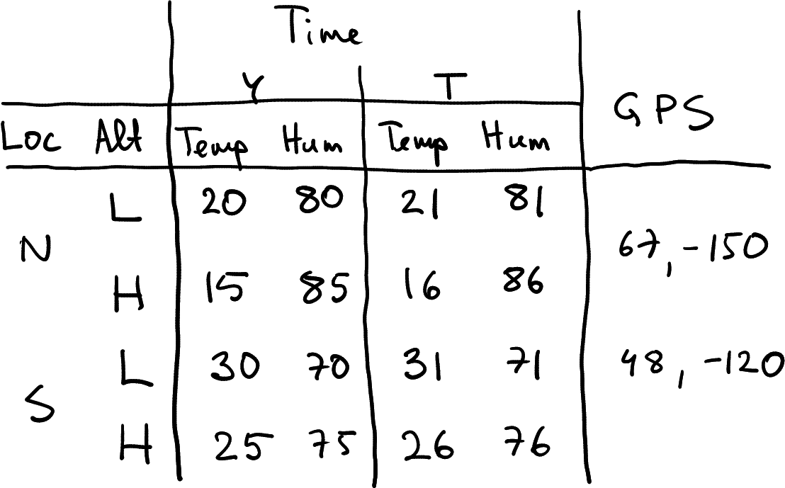
Temperature data with three groupings: location, altitude, and time. Here in a wide form with respect to altitude and time, and in long form with respect to location.
How might you store the data? The example table at right offers one option. You have stored two locations in two rows, and \(2\times 2\) altitude-time combinations in four columns.
Possible alternative ways to represent 3-way grouped data.
Why does your new task–store data over time–offer new ways to make the data frames? This is because now we have three grouping dimensions: location, altitude and time. And not surprisingly, more dimensions offer more ways to represent data. More specifically, tables (a), (b) and (c) are typically referred to as “wide form”, although all these tables have location in rows. Table (d) is pure long form, as the only columns are grouping indicators and the temperature values. Finally, (d) is pure wide form as no groupings are placed in rows. As in case of the two-grouping data, wide forms are often used to represent data visually, while the long form (d) is often useful for data processing. As above, the pure wide table (e) is rarely used, because it is cumbersome to process and display.
Exercise 15.16 Are these all possible options? Can you come up with more possible ways to represent these data? How many different ways are there in all to make a data frame of these data?
Temperature data as data cube.
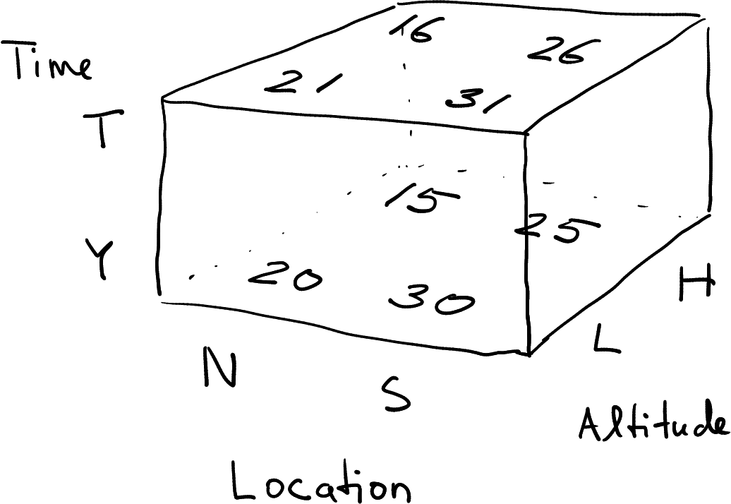
Finally, in case of three grouping dimensions, we can also represent data not as a rectangle but as a 3D “box”. This is commonly called data cube. Data cubes are not very common, and base-R does not support these. Data cubes are much harder to visualize, essentially you need to convert those to (2D) data frames to display their content. But they are actually used in exactly such context, when collecting 3D spatial data, or 4D spatio-temporal data. In the latter case we would need even a 4D cube. We do not discuss data cubes in this course. However, it is useful to know and imagine data cubes when reshaping data frames with multiple grouping dimensions.
15.2.4.2 Multiple values
But real data may be even more complicated. When you send your expensive weather balloons up, it is unlikely that you measure just temperature. You may measure a bunch of different atmospheric parameters, including humidity, wind speed, sunlight, gps coordinates and more.
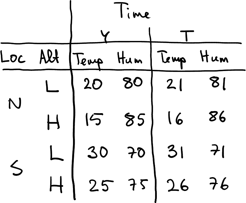
A possible representation of the atmospheric dataset that also contains humidity as a data frame.
First, imagine you also measure humidity. The dataset you collect may now look something like what is displayed at right. It is a data frame where rows represent location-altitude combinations, and columns represent time-measurement type combinations. How many grouping dimensions do we have in this data frame?
The answer is not quite obvious. We definitely have three–location, altitude and time. But will measurement type–temperature or humidity–also make it as a grouping dimension?
Temperature-humidity data in a completely long form.
This is not quite clear. From pure technical point of view, it is as
good as time or location, so you can imagine making a long form
dataset as seen here. But conceptually, this may not be a very useful
thing to do, as there are little need to use the value column for any
operations besides filtering it for either temperature or humidity.
These two are very different physical concepts, measured in completely
different units. You cannot easily put
them on the same figure, nor will computing averages, or filtering like
filter(value > 50) make much sense. So conceptually you probably do
not want to do that. It is more useful to just use two grouping
indicators–Location, Altitude and Time, and two value
columns: temperature and humidity.
Temperature-humidity data with geographic coordinates. The latter do not depend on time and elevation.
For instance, imagine you add the geographic coordinates to your weather data. The North and South mean large regions, so the small drift of your weather balloons does not matter much. The result may look like the table here at right.
Here I have just marked two sets of coordinates–one for North, one for South. This is because the coordinates do not depend on altitude and time (and they definitely do not depend on the type of measurement). Such partly constant values add some additional considerations when reshaping data. For instance, when converting the table at right to a data frame (the figure is just a handwritten table!), you need to replicate the GPS coordinates–you need to assign the same coordinates for both Low and High altitude. When converting the data frame to a long form, you probably want to add a column of coordinates to this dataset, one that contains largely identical values. This may be wasteful for large datasets.
Exercise 15.17
Consider the Ice Extent Data. Let’s only consider columns year, month, region, extent and area–remove columns data-type and time.- What are the grouping dimensions in these data?
- Are these in a wide form or in long form?
- What are values in these data? Do they change according along all the grouping dimensions? Would it make sense to combine the values into an additional grouping dimension?
- If you want to convert the dataset into a wide on by month, then what might the column names look like?
15.2.4.3 Reshaping multi-dimensional data
Now lets reshape a more complex dataset. Take the complete alcohol disorder data:
## # A tibble: 4 × 6
##   country   Code   Year disordersM disordersF population
##   <chr>     <chr> <dbl>      <dbl>      <dbl>      <dbl>
## 1 Taiwan    TWN    2019      0.903      0.258   23777742
## 2 Ukraine   UKR    2018      3.53       1.33    44446952
## 3 Taiwan    TWN    2018      0.892      0.259   23726186
## 4 Argentina ARG    2017      3.02       1.16    44054616
This dataset has three grouping dimensions–country, year and sex. It has two values, disorders (for males and females), and population. You can also easily see that population differs by country and year, but there is no separate population for males and females–it is a single population figure.
Are these data in a wide or in a long form? We can try to answer this in the following way:What does a row represent? Here, it is obviously a country-year combination. Hence it is in a long form according to country and year. Sexes are combined into the same row, hence it is in wide form according to sex.
What are the values? The data in the current form contain three value columns: male disorders, female disorders, and population. This means two types of values–disorder percentage (for both men and women), and population.
Year is not a value despite of being numeric–it is just a label on the time dimension.
What are the group indicators? It is fairly obvious that both country and year are groups. Moreover, country is given by two columns, country and Code, we might remove one and still have all the same information in data. So we have three group columns, one of which is redundant.
The final grouping dimension, sex, does not have a separate name, its name is embedded in the disorder column name.
Exercise 15.18 Consider a subset of COVID Scandinavia data. It looks like this:
read_delim("data/covid-scandinavia.csv.bz2") %>%
   select(code2, country, date, type, count, lockdown, population) %>%
   slice(c(201:204, 891:895, 2271:2274))
## # A tibble: 13 × 7
## code2 country date type count lockdown population
## <chr> <chr> <date> <chr> <dbl> <date> <dbl>
## 1 DK Denmark 2020-05-01 Confirmed 9311 2020-03-11 5837213
## 2 DK Denmark 2020-05-01 Deaths 460 2020-03-11 5837213
## 3 DK Denmark 2020-05-02 Confirmed 9407 2020-03-11 5837213
## 4 DK Denmark 2020-05-02 Deaths 475 2020-03-11 5837213
## 5 FI Finland 2020-05-01 Confirmed 5051 2020-03-18 5528737
## 6 FI Finland 2020-05-01 Deaths 218 2020-03-18 5528737
## 7 FI Finland 2020-05-02 Confirmed 5176 2020-03-18 5528737
## 8 FI Finland 2020-05-02 Deaths 220 2020-03-18 5528737
## 9 FI Finland 2020-05-03 Confirmed 5254 2020-03-18 5528737
## 10 SE Sweden 2020-05-01 Confirmed 22133 NA 10377781
## 11 SE Sweden 2020-05-01 Deaths 3027 NA 10377781
## 12 SE Sweden 2020-05-02 Confirmed 22432 NA 10377781
## 13 SE Sweden 2020-05-02 Deaths 3102 NA 10377781- What are the grouping dimensions in these data?
- Are these data in a long or a wide form?
- Would you count type (Confirmed/Deaths) as a grouping dimension?
- How many different values do you see in this dataset?
- Do all values change according to all dimensions?
- How would you describe the column code2? Is it value? Grouping dimension? Something else? Where would you put it when you’d transform the dataset into a wide form?
Let’s first convert the dataset into a long form, including long form by sex:
disordersL <- disorders %>%
   pivot_longer(starts_with("disorders"),
                           # all columns, names of which
                           # start with 'disorders'
                names_to = "sex",
                values_to = "disorders") %>%
   mutate(sex = ifelse(sex == "disordersF", "F", "M"))
                           # better code for sex
disordersL %>%
   head(10)
## # A tibble: 10 × 6
## country Code Year population sex disorders
## <chr> <chr> <dbl> <dbl> <chr> <dbl>
## 1 Argentina ARG 2015 43257064 M 3.07
## 2 Argentina ARG 2015 43257064 F 1.17
## 3 Argentina ARG 2016 43668236 M 3.04
## 4 Argentina ARG 2016 43668236 F 1.16
## 5 Argentina ARG 2017 44054616 M 3.02
## 6 Argentina ARG 2017 44054616 F 1.16
## 7 Argentina ARG 2018 44413592 M 3.04
## 8 Argentina ARG 2018 44413592 F 1.17
## 9 Argentina ARG 2019 44745516 M 3.11
## 10 Argentina ARG 2019 44745516 F 1.19Now the dataset is in the long form. Each row represents a country-year-sex combination, and we have four columns describing these grouping indicators (Code is redundant in the sense that it contains exactly the same information as country). We have two values: population and disorders. The representation is a little bit wasteful, as exactly the same population figure is replicated twice, once for men, once for women. But this data representation is good for many tasks, e.g. for comparing males and females on a barplot.
Alternatively, we may want to convert it into a form where country and sex are in rows, but years are in columns. In order to achieve this, we should first convert it into a long form (exactly what we just did), and thereafter make it into a wide form by year. Hence we need to spread the two value columns–population and disorders–into columns by year:
disordersL %>%
   pivot_wider(names_from = Year,
               values_from = c(population, disorders)) %>%
                           # note: both 'population' and 'disorders'
                           # are values
   head(4)
## # A tibble: 4 × 13
## country Code sex population_2015 population_2016 population_2017
## <chr> <chr> <chr> <dbl> <dbl> <dbl>
## 1 Argentina ARG M 43257064 43668236 44054616
## 2 Argentina ARG F 43257064 43668236 44054616
## 3 Kenya KEN M 46851496 47894668 48948140
## 4 Kenya KEN F 46851496 47894668 48948140
## population_2018 population_2019 disorders_2015 disorders_2016 disorders_2017
## <dbl> <dbl> <dbl> <dbl> <dbl>
## 1 44413592 44745516 3.07 3.04 3.02
## 2 44413592 44745516 1.17 1.16 1.16
## 3 49953300 50951452 0.747 0.744 0.742
## 4 49953300 50951452 0.654 0.655 0.658
## disorders_2018 disorders_2019
## <dbl> <dbl>
## 1 3.04 3.11
## 2 1.17 1.19
## 3 0.752 0.773
## 4 0.662 0.669Note that values_from takes a vector value, the names of the value
columns we want to combine into columns by year.
Exercise 15.19 Convert the alcohol disorders data into wide form, but this time the countries in columns, while keeping sex and year in rows.
What would you do with “iso2”?
Exercise 15.20 Take the Ice extent data. Let’s only consider columns year, month, region, extent and area–remove columns data-type and time.
- reshape the dataset in a way that there are only a single row for each year and region, and values for each month are in their separate columns.
- Reshape it into a wide form so that each year-month combination is in a single row, but North and South regions are in separate columns.
See the solution
15.2.5 Applications
Above we introduced reshaping. But there we assumed that you know what kind of shape you want the data to be in. This section provides a few examples that help you to decide what shape is appropriate for a particular task.
Consider the traffic fatalities data. It looks like
## # A tibble: 4 × 4
##    year state fatal      pop
##   <dbl> <chr> <dbl>    <dbl>
## 1  1984 OR      572 2675998.
## 2  1985 WA      744 4408994.
## 3  1985 OR      559 2686996.
## 4  1986 MN      571 4212996
This dataset has two groupings: year and state, and two values: number of fatalities, and population. It is stored in a long form.
You want to plot the traffic fatalities over time by state as a line plot with different colors denoting different states (see Section 14.4.2). Is this a good shape if you intend to use ggplot?
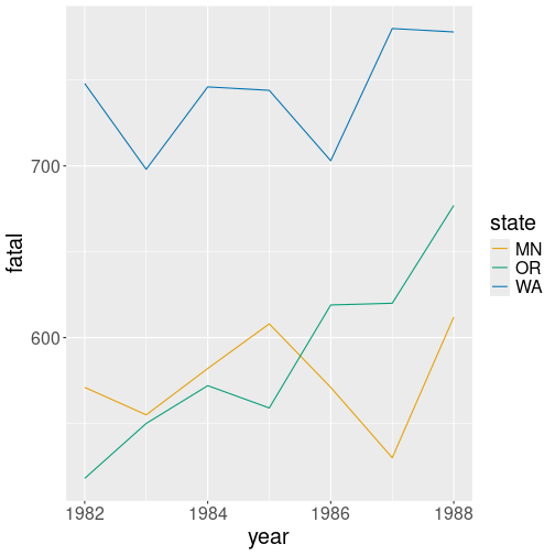
Traffic fatalities over time by state. Long form data is exceptionally well suited for ggplot.
The crucial part, when using ggplot, is the aesthetics mapping in
the form aes(x, y, col = ...). It turns out this is exactly the
form of data you want: aes(year, fatal, col = state) is designed for
long form data: it takes the fatal column, separates it by state, and
makes the lines in a separate color:
This is a good approach–it makes sense to let computer to figure out how many different states are there in the state column. It also makes sense to let us to decide which aesthetic we want to depend on state, maybe we want this to be line style instead of color.
Do you always want a long form data for such a plot? Well, it depends
on the software you are using. Not all software is designed to plot
data in long form. Base-R matplot(), for instance works
differently: you call it
matplot(x, Y, type = "l") where x is the vector of
x-values and Y is the matrix of y-values. This plots all
columns of Y against x. type = "l" asks it
to draw lines (otherwise it will be a scatterplot). Here we need
wide form data instead:
fWide <- fatalities %>%
   select(!pop) %>%
                           # all vars, except 'pop'
   pivot_wider(names_from = state,
               values_from = fatal)
head(fWide, 3)
## # A tibble: 3 × 4
## year MN OR WA
## <dbl> <dbl> <dbl> <dbl>
## 1 1982 571 518 748
## 2 1983 555 550 698
## 3 1984 582 572 746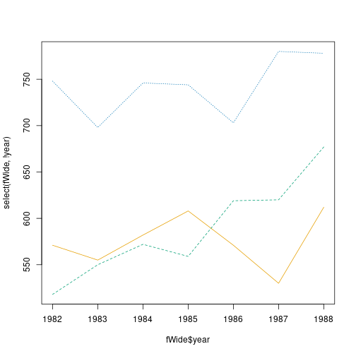
The same plot, made using base-R matplot(). This function expects
data in a wide form.
We also need to separate x, here the column year, and the data to be plotted (everything but year):
As you can see, the plot is basically the same, save the different fonts, line styles and such. Typically, ggplot is easier to use when you already have a ready-made dataset, but for plotting individual data vectors and matrices, base-R functions tend to be easier. As this example shows, it is also easier to use if your data is already in a wide form.
But now consider a somewhat different task: you want to do a trajectory plot (see Section 14.9.3.1) where fatalities in Oregon are on x-axis and fatalities in Washington on y-axis. Such plots are fairly common in many applications (although I have never seen it for traffic accidents). Here, unlike in the previous plot, a single point denotes both Oregon and Washington.
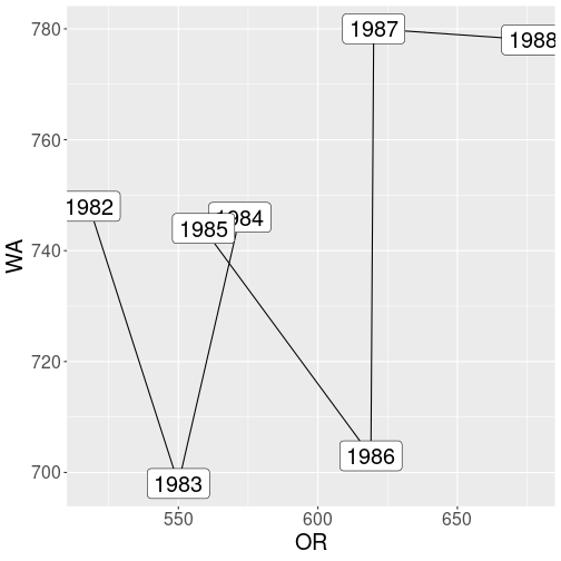
Traffic fatalities, Oregon versus Washington.
In order to use ggplot, you need something like aes(OR, WA).
However, there are not separate columns for OR and WA in the original
data. Hence we need to separate those–this type plot requires data
in
a wide
form. Here we can just re-use the wide table fWide we created
above:
Exercise 15.21 Use ice extent data. Both ice area and extent are certain surface areas that are measured in the same units (million km2 in these data) so you can put them on the same graph.
Make a line plot of ice extent and area over time, where time is on x-axis, and the two measures are on y axis.
15.3 Date and time
Date and time data is something we use a lot in the everyday life. However, it turns out that it is a surprisingly complex data type. Below, we work on a few common tasks with the related data structures.
A lot of the problems boil down to that the common time units like days, months, weeks, even minutes, are not physial units. Physical unit is just second with a precisely defined duration. The other units are convenience units, duration of which changes. Even more, time is commonly accounted with in a mixed measurement system, incorporating decimal, 12/24-based, 60-based, and 7-based units. Months, with their 28-31 day length, are an attempt to make moon’s revolution to fit into that of earth. On top of that, different regions have different time zones and daylight saving time, some of which is re-arranged each year. Not surprisingly, this creates a lot of issues when working with time data.
15.3.1 Duration
Consider a common task: you are analyzing the results of an athletic competition. There were four runners, and their time was:
| bib# | time |
|---|---|
| 102 | 58:30 |
| 101 | 59:45 |
| 104 | 1:00:15 |
| 103 | 1:02:30 |
So the the two best athletes run slightly below 1hr and the two slower ones slightly over that.
This is a common way to express the results. For time intervals less
than 1hr, we write MM:SS, e.g. 58:30. From the context we
understand what it means, in this case it is 58 minutes and 30 seconds
We can stay strictly within decimal system and physical units and write
3510 seconds instead, but unfortunately, such numbers are much
harder to understand than the everyday “58:30”.
We can load such data file into R as
This uses the fact that read_delim() can load not just files, but
also file content, fed to it as a string. So we write a multi-line
string that is just the content in the form or a csv file.
But now we have a problem: The results look like
## # A tibble: 4 × 2
##   `bib#` time
##    <dbl> <time>
## 1    102 58:30:00
## 2    101 59:45:00
## 3    104 01:00:15
## 4    103 01:02:30
As you can see, the entry “58:30” is not interpreted as 58 minutes and 30 seconds but as 58 hours and 30 minutes! The runners #102 and #102 apparently spent more than two days on the course! This can be confirmed by computing the time range:
## Time differences in secs
## [1]   3615 215100
Indeed the winner has time 3615 seconds (1h 15s, the runner #104), and the slowest one is 215100 seconds. That is what 59 hours and 45 mins amounts to.
In the small case here, it is easy to remedy the problem: we can just change “58:30” to “0:58:30”. But in larger data files, this is not feasible. We need to do this in the code. The strategy we pursue below is as follows: first, read the time column as text, then add “00:” in front of those columns that only contain a single colon, and finally, convert the result to duration.
First, we read data while telling the time has column type “character” (see documentation for details):
results <- read_delim(
   "bib#,time
102,58:30
101,59:45
104,1:00:15
103,1:02:30",
col_types = list(time = "character"))
                           # tell that column 'time' is of type 'character'
results
## # A tibble: 4 × 2
## `bib#` time
## <dbl> <chr>
## 1 102 58:30
## 2 101 59:45
## 3 104 1:00:15
## 4 103 1:02:30next, we can just use mutate() and ifelse() to add “00:” in front
of the columns that contain a single colon only:
## # A tibble: 4 × 2
##   `bib#` time
##    <dbl> <chr>
## 1    102 00:58:30
## 2    101 00:59:45
## 3    104 1:00:15
## 4    103 1:02:30
This code:
- counts the colons in the column time:
str_count(time, ":") - if there is a single colon, pastes “00:” in front of the value
paste0("00:", time) - otherwise keeps time as it is (just
time)
Now all the time column values have hour markers in front of minutes,
but the column is still of character type, not time. We can convert
it to time using parse_time()
function from the readr package:
results <- results %>%
   mutate(time = ifelse(str_count(time, ":") == 1,
                        paste0("00:", time),
                        time)) %>%
   mutate(time = parse_time(time))
Obviously, we can achieve the same in a single mutate.
Now the time is understood in a correct manner: the winner is
## # A tibble: 1 × 2
##   `bib#` time
##    <dbl> <time>
## 1    102 58'30"
15.4 More about data cleaning
This section gives examples of different data cleaning tasks. It tries to focus on tasks and tools that are more common or generalize better. But data can be messy in many many ways, so it does not pay off to even attempt to be comprehensive.
15.4.1 Separate a single column into multiple columns
A common problem with many datasets is that a single column combines multiple values that need to be handled separately. For instance, Dawgs Dash race age and sex into a single column in the form “40 | F” for 40-year old females. If you are interested to analyze the participants age and gender, you need to separate these two values.
15.4.1.1 “Any Drinking” data in long form
Below, I am using a different dataset–Any drinking–that results in awkward combination of year and sex when you reshape it.
Any Drinking dataset looks as follows:
## # A tibble: 3 × 8
##   state    location        both_sexes_2008 females_2008 males_2008 both_sexes_2012
##   <chr>    <chr>                     <dbl>        <dbl>      <dbl>           <dbl>
## 1 Virginia Surry County               41.1         31.3       51.3            41.8
## 2 Arkansas Woodruff County            37.6         28.2       47.2            37.6
## 3 Nebraska Thurston County            37.8         30         46              36.8
##   females_2012 males_2012
##          <dbl>      <dbl>
## 1         32.6       51.3
## 2         28.2       47.3
## 3         29.3       44.5
As you can see, the dataset is in a wide form with two groupings, year and sex, combined into columns. The values represent the drinking prevalence, the percentage of the respective population who had consumed at least one alcoholic drink during the preceding 30 days. (See Section 15.2 for more about wide form and long form data, and reshaping.) We may want convert it into a long form with columns “county”, “sex”, “year”, and “prevalence” for easier filtering and other operations. So after reshaping we have
lDrinking <- drinking %>%
   pivot_longer(!c(state, location),
                names_to = "sexyear",
                values_to = "prevalence")
lDrinking %>%
   head(8)
## # A tibble: 8 × 4
## state location sexyear prevalence
## <chr> <chr> <chr> <dbl>
## 1 Virginia Surry County both_sexes_2008 41.1
## 2 Virginia Surry County females_2008 31.3
## 3 Virginia Surry County males_2008 51.3
## 4 Virginia Surry County both_sexes_2012 41.8
## 5 Virginia Surry County females_2012 32.6
## 6 Virginia Surry County males_2012 51.3
## 7 Arkansas Woodruff County both_sexes_2008 37.6
## 8 Arkansas Woodruff County females_2008 28.2This dataset is in a long form, but unfortunately, year and sex are combined in a rather awkward way. We want to replace sexyear with two columns: sex and year.
Below, we perform these tasks using regular expressions (regexps) (see
Section 7.5). Although tidyr offer dedicated
functions (various separate_...()-functions), it is more valuable to
learn about regular expressions as these generalize to many more tasks
and programming languages.
15.4.1.2 Extract year
Regular expressions operate on various patterns in the text, and they include quite powerful tools to describe the patterns. In order to separate year, there are multiple options:
- delete everything that is not a number
- separate the last four characters
- delete everything till (and including) the last underscore _
Below I demonstrate all these operations.
15.4.1.2.1 Deleting everything that is not a number.
You can spot a number using the [:digit:] character class
(see Section 7.5.2), and everything that is not
a number as [^[:digit:]]. Hence, any number of non-digits is
[^[:digit:]]*, that should be replace with nothing, i.e. with the
empty string. As there is only one substitution to be made, you can
use both sub() or gsub().
Here is an example:
## [1] "1234"Now we can use this idea for transforming the column:
## # A tibble: 5 × 5
##   state    location     sexyear         prevalence  year
##   <chr>    <chr>        <chr>                <dbl> <dbl>
## 1 Virginia Surry County both_sexes_2008       41.1  2008
## 2 Virginia Surry County females_2008          31.3  2008
## 3 Virginia Surry County males_2008            51.3  2008
## 4 Virginia Surry County both_sexes_2012       41.8  2012
## 5 Virginia Surry County females_2012          32.6  2012
This approach creates a new column year by deleting everything that is not a number, and converts it into a number (otherwise it would be a string).
15.4.1.2.2 Separate the last four characters
Any character can be marked by a dot ., and end of the string is
denoted by $. So the last four characters are ....$. This makes
it easy to remove the last four characters:
## [1] "both_sexes_"However, the task here is the opposite–remove everything, except the
last four characters. As a solution I propose to combine the last
four chracters with everything: .* (any number of any characters),
and replace this with the last four characters. This is equivalent
with removing everything else.
- First, the regexp for “everything, followed by four characters at
the end of string” is
.*....$. - However, the problem with this
regexp is that it does not let you to use its last part,
....$for replacement. You need the put the latter into parenthesis(....)$to denote match groups. So the actual regexp will look like.*(....)$.
- Now you can refer to this match group
(....)as\1, the first match group. - But because
\is a special symbol withing strings, you need either to escape it with another\, or alternatively to use raw strings. I’ll take the latter approach.
So the final approach will be
## [1] "1234"