K Exercise solutions
K.1 Find your files
K.1.1 File system tree
K.1.1.1 Sketch your file system tree
This is, obviously, different for everyone, but here is mine: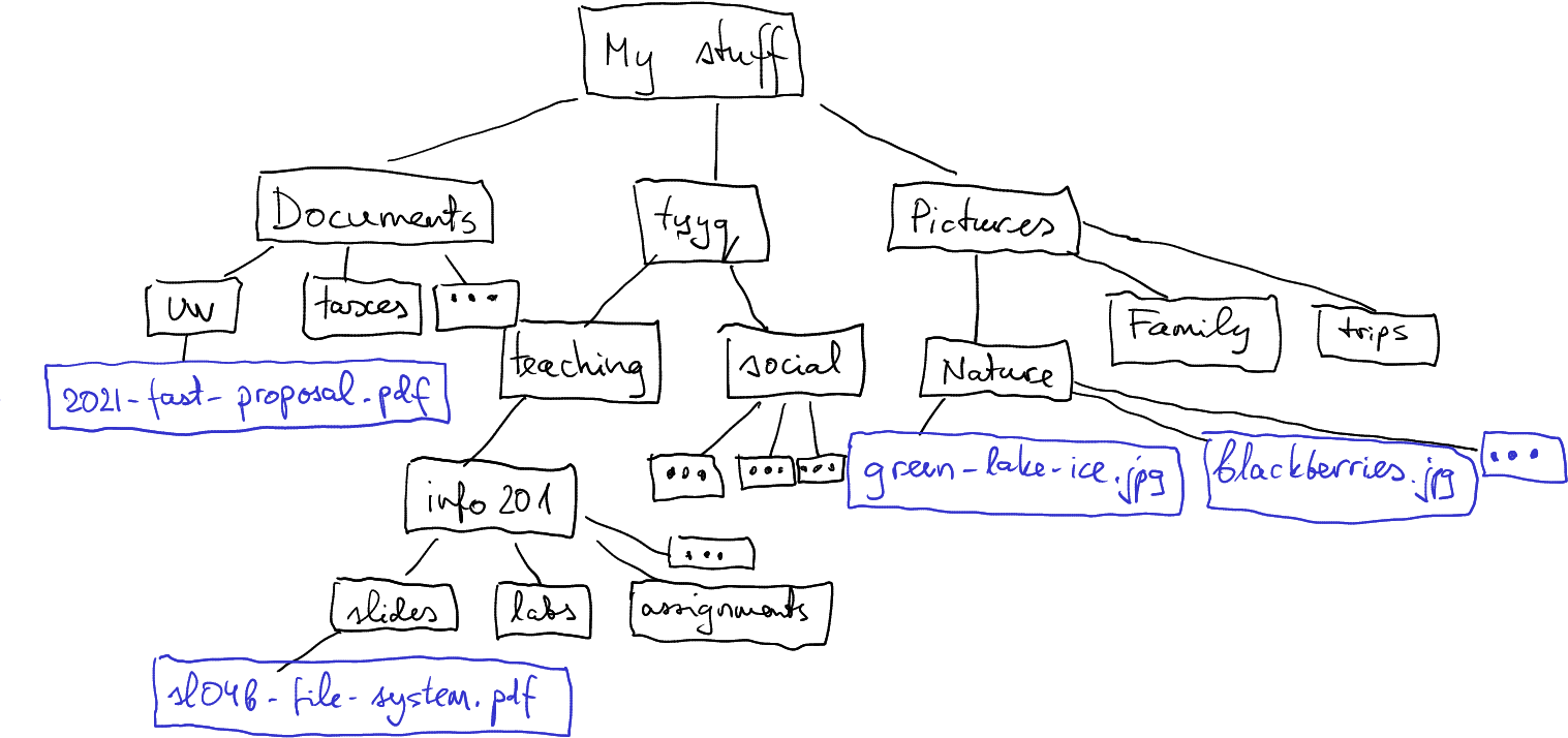
A subset of the file system tree in my computer. Black boxes denote folders, orange boxes are files within the folders.
K.1.1.2 Sketch your picture folder tree
Here is mine. I have picked mostly shorter example names, just to fit those on the figure.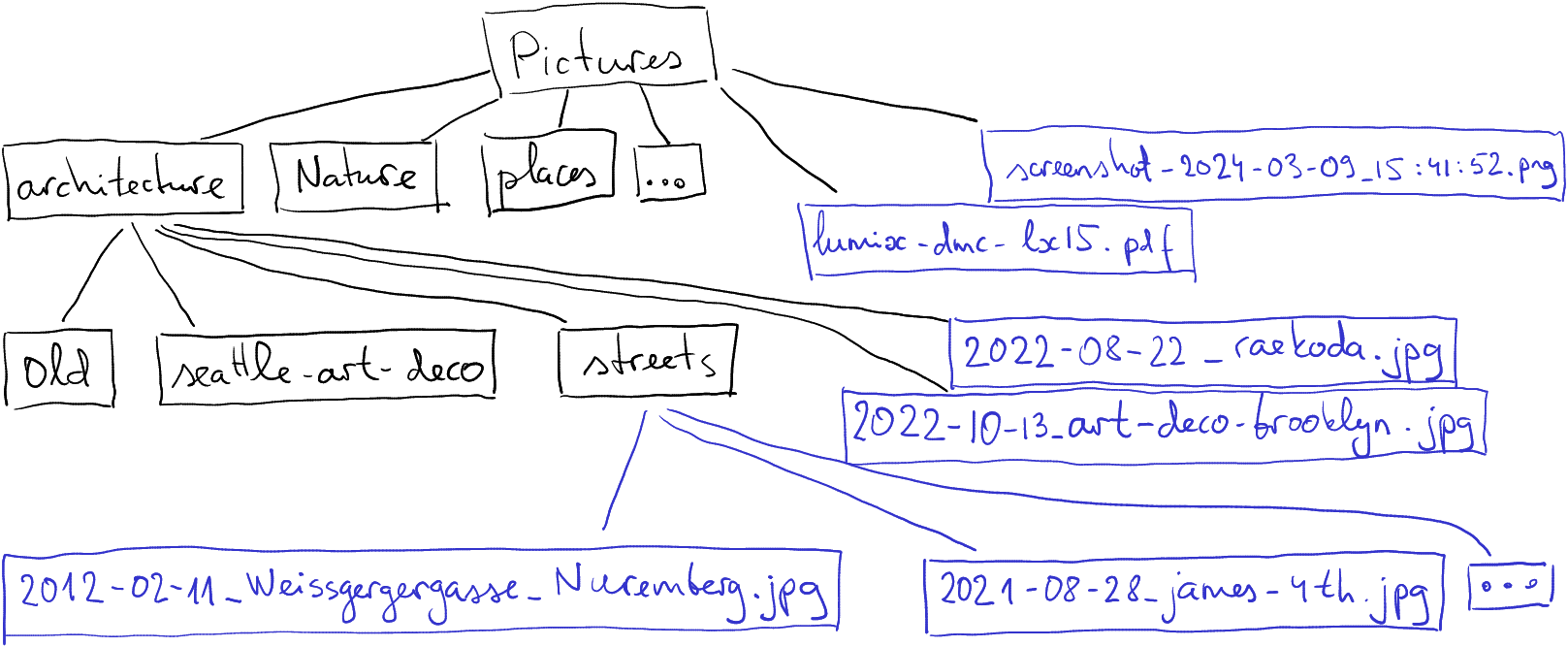
A subset of the Pictures folder in my computer. Black boxes denote folders, blue boxes are files.
K.1.1.3 Navigate the file tree
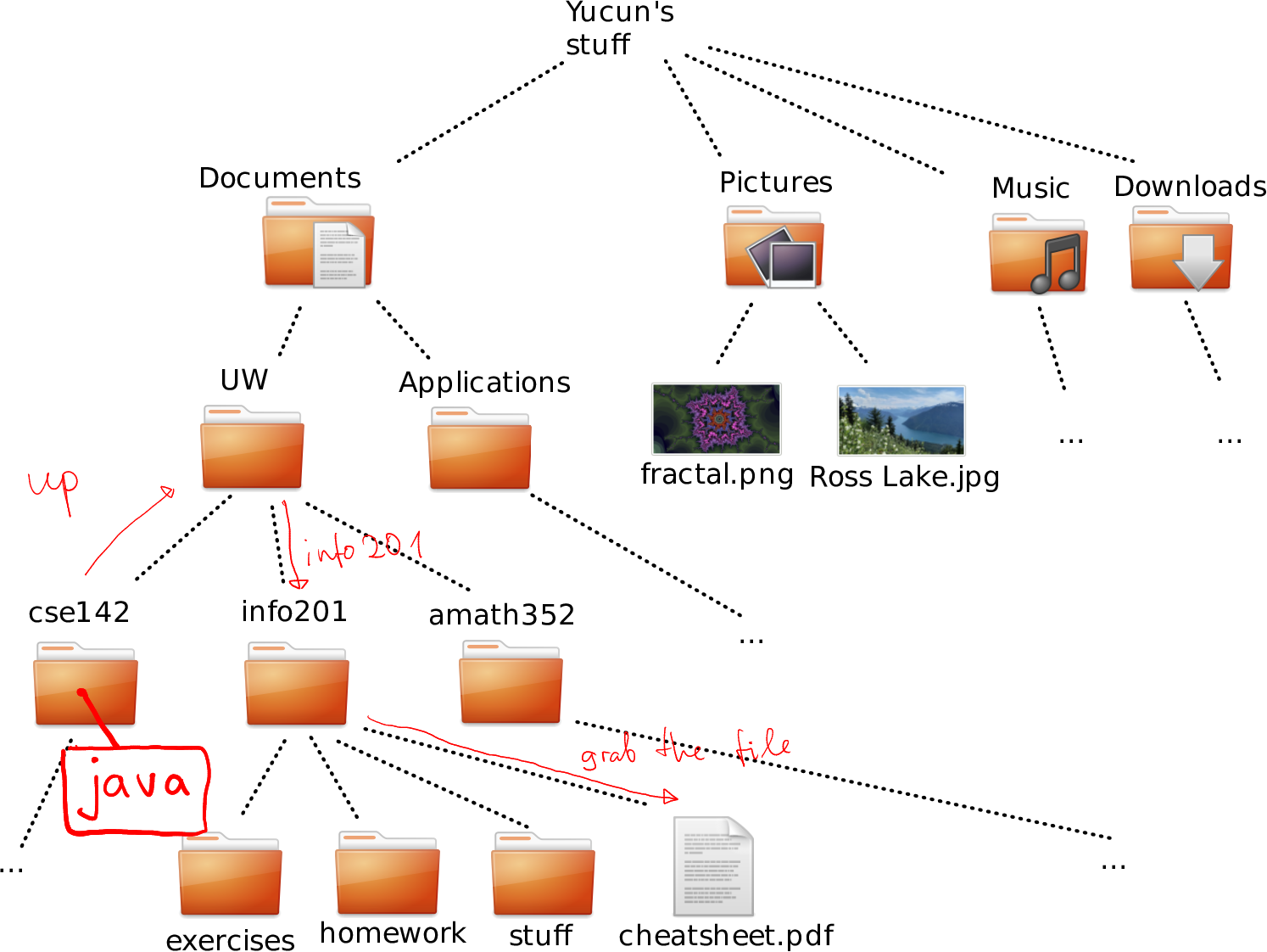
How to navigate to cheatsheet.pdf from cse142.
From cse142 to cheatsheet.pdf we can move as (see the figure):
- up (into UW)
- into info201
- grab cheatsheet.pdf from there
Or in the short form:
"../info201/cheatsheet.pdf"Note that we should not start be going up to cse142 as we already are there.
K.1.1.4 Matlab accessing matrix.dat
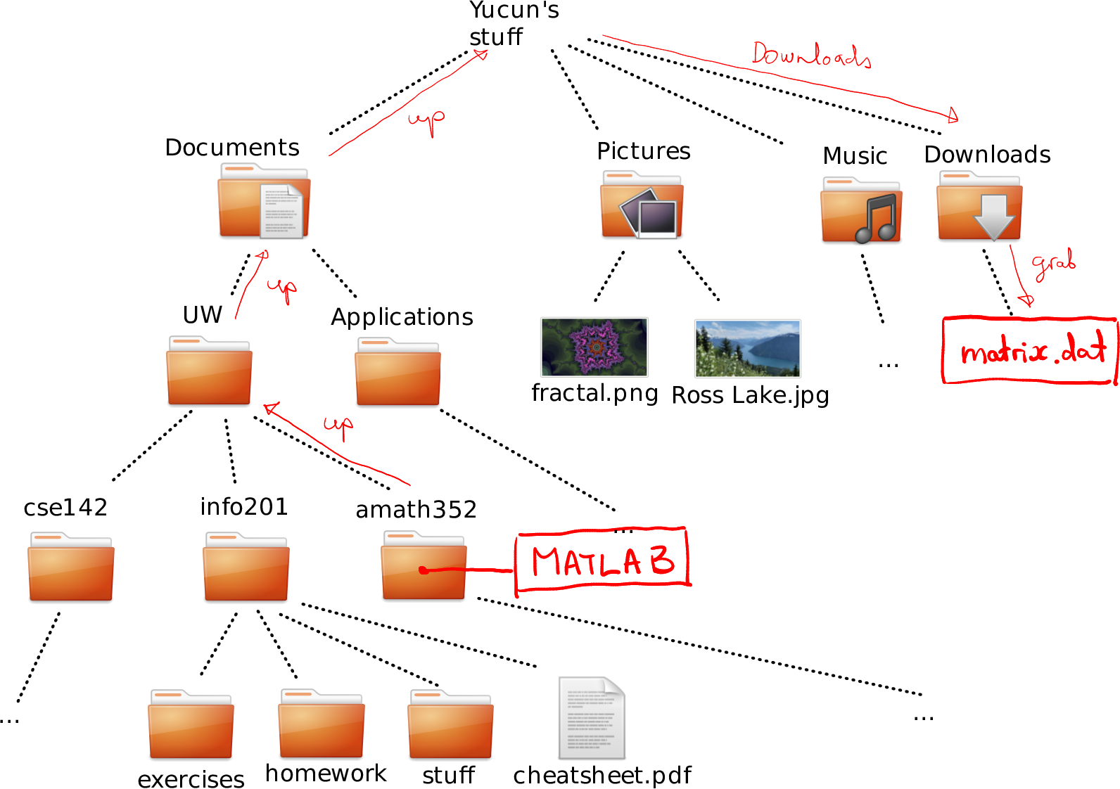
How to navigate to cheatsheet.pdf in Downloads from amat352.
From amath352 to matrix.dat we can move as (see the figure):
- up (into UW)
- up (into Documents)
- up (into Yucun’s stuff)
- into Downloads
- grab matrix.dat from there
Or in the short form:
"../../../Downloads/matrix.dat"Again, we should not start be going up to amath352 as we already are there.
K.1.1.5 lab1.md from exercises
Because R’s working directory is already inside the same folder as the file, you can just tell that
- grab lab1.md
In the computer form, the relative path is just
lab1.md
This is because there is no need to go up, down, or anywhere else. Just the file name is enough.
K.1.1.6 Get picture from info201
Again, this is different on your computer. But given my file system tree looks like above, my path will be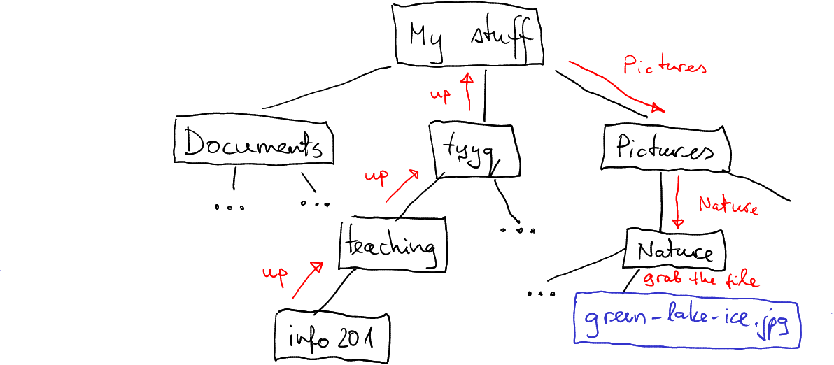
How I can access green-lake-ice.png from my info201 folder.
- up (to teaching)
- up (to tyyq)
- up (to my stuff)
- into Pictures
- into Nature
- grab the green-lake-ice.jpg from there.
In the short form, it is
"../../../Pictures/Nature/green-lake-ice.jpg"Note that I do not have pictures in Pictures folder, but in subfolders inside there. If you do, the descent into Nature will be unnecessary.
K.1.1.7 Absolute path
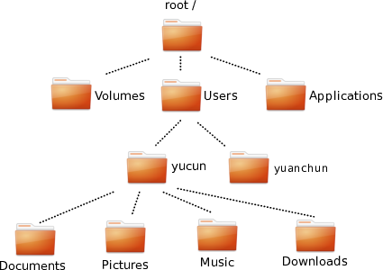
For reference, here is the file system tree again.
Now the initial location (the working directory of the java program) is irrelevant. One has to to start from root:
- Start at root “/”
- into “Users”
- into “yucun”
- into “Pictures”
- grab “Ross Lake.jpg” from there
Or in the computer way:
/Users/yucun/Pictures/Ross Lake.jpgK.1.1.8 Absolute path of an image
Suppose I have an image “fractal.png” inside of my Picture folder that, in turn, is in my home folder. Assume further that I am using Windows and my home folder is on “D:” drive. The long directions might look like:
- start at root “This PC”
- go to drive “D:”
- go to “Users”
- go to “siim” (assume “siim” is my user name)
- go to “Pictures”
- grab “fractal.png” from there.
In the short form it is
D:/Users/siim/Pictures/fractal.png
Note that we do not use the root “This PC” when writing paths on windows.
K.1.1.9 Absolute path of the home folder
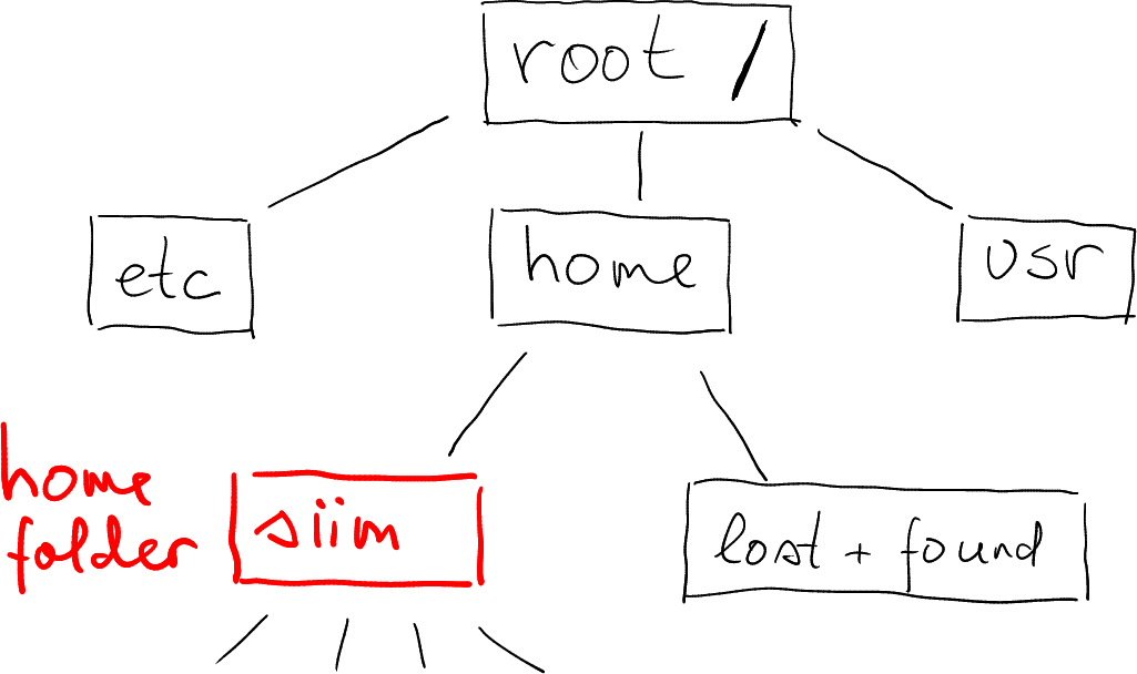
Obviously, this is different for every user and every computer. Here is mine on my home computer. I have marked a few other folder (etc, system configuration files and usr – installed applications).

Absolute path, here root - home - siim, as shown in Gnome file selector.
There are multiple ways to see where in the file system tree it is located, one option is to use file managers. Here is an example that shows the path in Gnome file selector. Note that root is denoted by a hard disk icon, and the home folder siim is combined with a home icon.
K.1.1.10 Yucun moving his project
- If he is using absolute path (it might be
"/Users/yucun/Documents/data/data.csv"), the it does not change. This is because absolute path always starts from the file system root, and file system root does not change if you move around your files and folders–as long as the file in question (data.csv) remains in place. - If he moves data to a different computer… then he probably has
to change the paths. Most importantly, the other computer may not
have the data folder inside of the Documents folder, but
somewhere else. Second, the other computer may also have different
file system tree, e.g. if the other one is a PC, his home folder
may be
"C:/Users/yucun"instead. Relative path is of no help here, unless the other computer has similar file and folder layout.
K.2 Introduction to R
K.2.1 Variables
K.2.1.1 Invalid variable names
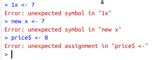
K.2.2 Data Types
K.2.2.1 Years to decades
If we integer-divide year by “10”, then we get the decade (without the trailing “0”). E.g.
## [1] 196Now we just multiply the result by 10:
## [1] 1960Or, to make the order of operation more clear:
## [1] 2020K.2.2.2 Are you above 20?
There are many ways to do it, here is just one possible solution:
## [1] TRUENote the variable names: age is fairly self-explanatory, older is
much less so. In complex projects one may prefer name like
age_over_20 or something like this. But in a few-line scripts, even
a and o may do.
K.2.3 Producing output
K.2.3.1 Sound around earth
We can follow the lightyear example fairly closely:
s <- 0.34  # speed of sound, km/s
distance <- 42000
tSec <- distance/s
tHrs <- tSec/3600
tDay <- tHrs/24
cat("It takes", tSec, "seconds, or",
    tHrs, "hours, \nor", tDay,
    "days for sound to travel around earth\n")
## It takes 123529.4 seconds, or 34.31373 hours,
## or 1.429739 days for sound to travel around earthNote how we injected the new line, \n in front of “or” for days.
This makes the output lines somewhat shorter and easier to read.
Now it does not happen often that sound actually travels around the world, but the pressure wave of Krakatoa volcanic eruption 1883 was actually measured circumnavigating the world 3 times in 5 days. See the Wikipedia entry.
K.3 Functions
K.3.1 For-loops
K.3.1.1 Odd numbers only
The form of seq() we need here is seq(from, to, by) so that the
sequence runs from from to to with a step by. So we can write
## 1^2 = 1
## 3^2 = 9
## 5^2 = 25
## 7^2 = 49
## 9^2 = 81
K.3.1.2 Multiply 7
We can just follow the loop example in Section 5.1:
## 7*10 = 70
## 7*9 = 63
## 7*8 = 56
## 7*7 = 49
## 7*6 = 42
## 7*5 = 35
## 7*4 = 28
## 7*3 = 21
## 7*2 = 14
## 7*1 = 7
## 7*0 = 0
Note the differences:
- we go down from “10” to “0” using
10:0 - we need specify that the numbers and strings we print should not be
separated by space using
sep=""argument for cat. - we could have created a separate variable
i7 <- i*7but we chose to write this expression directly as an argument forcat().
K.3.1.3 Print carets ^
This is very simple: we just need to use cat("^") 10 times in a
loop:
## ^^^^^^^^^^Note that we end the line after the loop, this is because we do not want the whatever-follows-it to be on the same line.
K.3.1.4 Asivärk
The trick here is to use the caret-printing example, but now we need to do it not 10 times, but a different number of times on each line. So first let’s write the outer loop that just prints 10 lines of a single caret:
## ^
## ^
## ^
## ^
## ^
## ^
## ^
## ^
## ^
## ^
But now we do not want to print the single caret–you want to print a different number of carets in each line. Let’s call this number nCarets. For asivärk, nCarets should just be equal to the line number, line. Now we can use the caret-printing example, but printing nCarets instead of 10 carets:
for(line in 1:10) {  # do 10 lines
   nCarets <- line
   for(i in 1:nCarets) {  # do nCaret carets
      cat("^")
   }
   cat("\n")  # done with the line, do new line
}
## ^
## ^^
## ^^^
## ^^^^
## ^^^^^
## ^^^^^^
## ^^^^^^^
## ^^^^^^^^
## ^^^^^^^^^
## ^^^^^^^^^^Note how the middle rows are essentially the
caret-printing example, the only difference is
1:n instead of 1:10 in the loop header. This ensures that the
outer loop index n can change the number of carets printed.
We also need to keep the new line (cat("\n"))
separate from printing on the same row, that’s why it is put outside
of the caret-loop.
K.3.1.5 Inverted asivark
This is very similar to the original asivärk (Section @ref(sol-fn-loop-asivärk)), just now the number of bars on line is not the same as line number. In the image contains 7 lines, and on the 1st line there are 7 bars, 2nd line there are 6 bars and down to a single bar on the 7th line. Here you can find the correct number of bars as nBar = 8 - line:
for(line in 1:7) {  # do 7 lines
   nBars <- 8 - line
   for(i in 1:nBars) {  # do nBar bars
      cat("|")
   }
   cat("\n")  # done with the line, do new line
}
## |||||||
## ||||||
## |||||
## ||||
## |||
## ||
## |Everything else is the same as in the original asivärk.
K.3.1.6 Combined asivärk
Here we combine both the ordinary (Section K.3.1.4) and the inverted asivärk (Section K.3.1.5). On each line we need to print nBars bars and nOs “o”-s. As above, we have nBars = 7 - line and nOs = line:
for(line in 1:7) {
   nBars <- 8 - line
   for(i in 1:nBars) {
      cat("|")
   }
   nOs <- line
   for(i in 1:nOs) {
      cat("o")
   }
   cat("\n")
}
## |||||||o
## ||||||oo
## |||||ooo
## ||||oooo
## |||ooooo
## ||oooooo
## |oooooooK.3.1.7 Wide asivärk
We follow exactly the same approach as for the normal asivärk (Section K.3.1.4), we’ll count lines, and for each line, we’ll figure out how many “o”-s to print. In the 1st line you need 1, in the second line you need 3, 3rd line has 5, and so on. It is easy to see that here nOs = 2 nLines - 1:
for(line in 1:7) {  # count lines
   nOs <- 2*line - 1  # number of 'o'-s per line
   for(i in 1:nOs) {
      cat("o")
   }
   cat("\n")
}
## o
## ooo
## ooooo
## ooooooo
## ooooooooo
## ooooooooooo
## oooooooooooooK.3.1.8 Mountain in rain
This amounts to combine an inverted asivärk (Section K.3.1.5), a wide asivärk (Section K.3.1.7), and another inverse asivärk in a similar fashion as the combined asivärk (Section K.3.1.6). The outer loop counts lines, and for each line we need to compute how many bars and “o”-s we need to print:
for(line in 1:7) {
   nBars <- 8 - line
   for(i in 1:nBars) {
      cat("|")
   }
   nOs <- 2*line - 1  # number of 'o'-s per line
   for(i in 1:nOs) {
      cat("o")
   }
   for(i in 1:nBars) {
      cat("|")
   }
   cat("\n")
}
## |||||||o|||||||
## ||||||ooo||||||
## |||||ooooo|||||
## ||||ooooooo||||
## |||ooooooooo|||
## ||ooooooooooo||
## |ooooooooooooo|K.3.1.9 Pick three best apples
Here the trick is to find which apples are the best. You can evaluate their goodness while still on ground, or maybe rather pick it up and check if any of those you have in hand is worse than the new one. And if it is, drop the old one and keep the new one. The task list might look like:
Pick the 3 first apples
for(all other apples you see) {
   pick the apple
   is it better than any of those you have in hand?
   if yes, then drop your worst apple and keep the new one
}
Now you have the 3 best apples in hand.
Note that here we initally pick just three first apples without any checks, and first thereafter we’ll start comparing the new and old apples.
This is essentially a similar accumulation task, just the accumulation process is now somewhat different because we only can keep three apples at time.
K.3.1.10 \(1/1 \times 1/2 \times \dots\)
- As the task is to multiply fractions, the accumulating process here means multiplication. So instead of dropping berries in the basket, we multiply numbers.
- For multiplication, we should start with value “1”. This is because it will not change the first element we accumulate.
So the code might look like:
## [1] 2.755732e-07K.3.3 Writing functions
K.3.3.1 M87 black hole in km
The function might look similar to feet2m, but we may need to
compute the length of a single light-year inside of the function:
ly2km <- function(distance) {
   c <- 300000
   ly <- c*60*60*24*365  # length of a single light-year:
                           # speed of light * seconds in minute *
                           # minutes in hour * hours in day *
                           # days in year
   distance*ly
}
And we find the distance to the black hole as
## [1] 5.20344e+20or maybe it is easier to write it as
## [1] 5.20344e+20If this number does not tell you much then you are not alone–so big distances are beyond what we one earth can perceive.
K.3.3.2 Years to decades
Perhaps the most un-intuitive part here is the integer division %/%:
it just divides the numbers, but discards all fractional parts. For
instance,
## [1] 202In order to make this into the decade, we just need to multiply the result by 10 again. So the function might look like:
## [1] 2020## [1] 1930## [1] 1960## [1] 1970K.3.3.3 Dates
## [1] "2012-3-30"## [1] "2025-3-30"Note that the order of arguments is somewhat arbitrary, you can also
use function(month, day, year) or any other order. But obviously,
later you need to supply the actual arguments in the corresponding order.
K.3.3.4 Output versus return
We can create such a function by just using paste0:
hi <- function(name) {
   paste0("Hi ", name, ", isn't it a nice day today?")
                           # remember: paste0 does not leave spaces b/w arguments
}
This function returns the result of paste0, the character string
that combines the greeting and the name. It does not output
anything–there is no print nor cat command. We can show it works
as expected: when called on R console, its returned value, the
greeting, is automatically printed:
## [1] "Hi Arthur, isn't it a nice day today?"and if the result is assigned to a variable then nothing is printed:
K.3.3.5 Asivärk with different letters
The function is made of the asivärk for-loop (see Section K.3.1.4). The modifications are simple:- move the code inside a function–here called asivärk, but you may prefer to use a name that does not contain “ä”.
- decide the argument names. Here nLines for the desired number of lines and letter for the desired letter.
- Replace the hard-coded 10 lines and caret “^” with the arguments.
- To ensure that the function does not return anything, we’ll
explicitly return
NULL. This is the closest thing to “nothing” there is in R.
asivärk <- function(nLines, letter) {
   for(line in 1:nLines) {
      nLetters <- line
      for(c in 1:nLetters) {
         cat(letter)
      }
      cat("\n")
   }
   return(NULL)
}
(Instead of return(), you can use the function of invisible().
This returns the value invisibly, i.e. it does not print it on
screen.)
You can call it as
## 😀
## 😀😀
## 😀😀😀
## 😀😀😀😀## NULLK.4 Vectors
K.4.1 Vectorized operations
K.4.1.1 Extract April month row numbers
We just need to make a sequence from 3 till no more than 350 (number of rows) with step 12:
##  [1]   3  15  27  39  51  63  75  87  99 111 123 135 147 159 171 183 195 207 219 231
## [21] 243 255 267 279 291 303 315 327 339
K.4.1.2 Yu Huang and Guanyin in liquor store
We can just call the data age and cashier:
In normal language–you are able to buy if you are at least 21 years old or your cashier is Guanyin. This means the first customer cannot, but the other two can buy the drink.
The expression is pretty much exactly the sentence above, written in R syntax:
## [1] FALSE TRUE TRUENote that we use >= to test age at least 21, and == to test
equality.
So the first customer cannot get the drink but the two others can.
K.4.1.3 Descriptive statistics
## [1] 5.5## [1] 5.5## [1] 5.5So all averages are the same.
## [1] 5.5## [1] 5.5## [1] 1Medians of x and y are the same, but that of z is just 1.
## [1] 1 10## [1] -11 22## [1] 1 55Here range is easily visible from how the vectors were created, so computation is not really needed. But this is usually not the case where the vectors originate from a large dataset.
## [1] 9.166667## [1] 99.16667## [1] 243Variances are hard to judge manually, but they are different too.
So we summarized these vectors into five different numbers (two for range), despite of the fact that they were of different length.
K.4.1.4 Recycling where length do not match
## Warning in c(10, 20, 30, 40) + 1:3: longer object length is not a multiple of
## shorter object length
## [1] 11 22 33 41This is the warning message, as you can see, this operations results
in an incomplete recycling where only the first component 1 of the
shorter vector was used.
K.4.2 Vector indices
K.4.2.2 Extract positive numbers
We have data
height <- c(160, 170, 180, 190, 175)  # cm
weight <- c(50, 60, 70, 80, 90)  # kg
name <- c("Kannika", "Nan", "Nin", "Kasem", "Panya")
Height of everyone at least 180cm:
## [1] 180 190Names of those at least 180cm:
## [1] "Nin" "Kasem"Weight of all patients who are at least 180cm tall
## [1] 70 80Names of everyone who weighs less than 70kg
## [1] "Kannika" "Nan"Names of everyone who is either taller than 170, or weighs more than 70.
## [1] "Nin" "Kasem" "Panya"K.4.2.3 Character indexing: state abbreviations
First, we can set names to the state.abb variable:
Note that we need to be sure that the names and abbreviations are in the same order! (They are, this is how the data is defined, see Section I.20.) This results in a named vector:
##    Alabama     Alaska    Arizona   Arkansas California
##       "AL"       "AK"       "AZ"       "AR"       "CA"
Now we can just extract the abbreviations:
##        Utah Connecticut      Nevada
##        "UT"        "CT"        "NV"
This is a common way to create lookup tables in R.
K.4.3 Modifying vectors
K.4.3.1 Wrong number of items
Feeding in a single item works perfectly:
## [1] "backpack" "ipad" "ipad"Just now both the elements 2 and 3 are “ipad”. This is because of the recycling rules (see Section 6.3.4), the shorter item (here “ipad”) will just replicated as many times as needed (here two).
But feeding in 3 elements results in a warning:
## Warning in supplies[c(2, 3)] <- c("tablet", "book", "paper"): number of items to
## replace is not a multiple of replacement length## [1] "backpack" "tablet" "book"Otherwise, the replacement works, just the last item, “paper”, is ignored.
K.4.3.2 Absolute value
We can do it explicitly in multiple steps:
x <- c(0, 1, -1.5, 2, -2.5)
iNegative <- x < 0  # which elements are negative
positive <- -x[iNegative]  # flip the sign for negatives
                           # so you get the corresponding
                           # positives
x[iNegative] <- positive  # replace negatives
x
## [1] 0.0 1.0 1.5 2.0 2.5However, it is much more concise if done in a shorter form:
## [1] 0.0 1.0 1.5 2.0 2.5K.4.3.3 Managers’ rent
Here is the data:
income <- c(Shang = 1000, Zhou = 2000, Qin = 3000, Han = 4000)
rent <- c(Shang = 200, Zhou = 1000, Qin = 1700, Han = 2800)
This problem can be solved in two ways. First the way how it is stated in the problem:
b <- c(0, 0, 0, 0)  # to begin with, befit "0" for everyone
iHR <- rent > 0.5*income  # who is rent-burdened?
iHR  # just for check
## Shang Zhou Qin Han
## FALSE FALSE TRUE TRUESo Qin and Han are rent-burdened.
## [1] 0 0 425 700Here we replaced benefits for two people–we had to use iHR on both sides of the assignment.
We can also solve it the other way around (not asked in the problem statement): first we can compute the benefit for everyone, and thereafter replace it for the non-rent burdened with “0”:
b <- 0.25*rent  # benefits to everyone
iLR <- rent <= 0.5*income  # who's rent is low?
b[iLR] <- 0  # replace their benefits by 0.
b
## Shang Zhou Qin Han
## 0 0 425 700Note that all replacement elements have the same value here, “0”.
K.5 Working with strings
K.5.1 Base-R string function
K.5.1.1 Combining three kings
Whe have three titles and names:
We need to proceed in three steps:- combine title and names with a space in-between
- combine first and second titles/names with a comma in-between. This
should be done with the
collapse =argument, as we combine elements in the same string vector. - combine this with the last title/name with “and” in-between. This
should be done with
sep =argument, as on both sides we now have lenght-1 vectors.
The code might look like:
## [1] "king Darius" "shahanshah Ardashir" "shah Soleiman"## combine 1st and 2nd persons,
## separated with comma
titlename12 <- paste(titlename[1:2], collapse = ", ")
titlename12## [1] "king Darius, shahanshah Ardashir"## [1] "king Darius, shahanshah Ardashir and shah Soleiman"For comparison, here is how to achieve the same result with
str_flatten_comma() from stringr package:
## [1] "king Darius, shahanshah Ardashir and shah Soleiman"or with using pipes:
## [1] "king Darius, shahanshah Ardashir and shah Soleiman"See the documentation for more details.
K.5.1.2 Secure http
This is a strightforward application of grep():
addresses <- c("www.urban.org", "file:///home/otoomet/",
               "https://faculty.washington.edu/",
               "http://www.example.com/",
               "https://www.index.ie", "http://tartu.edu")
grep("https:", addresses, value = TRUE)
## [1] "https://faculty.washington.edu/" "https://www.index.ie"You need to specify value = TRUE for grep() to return the actual
addresses.
Note that you may want to use regular expressions, e.g. “^https:” to specify that the “https:” string must be in the beginning of the string.
K.5.1.3 Boats and ships
This is a straightforward application of sub():
## [1] "steamship" "sailship" "motorship" "river ship"Note that both “boat” and “ship” are treated as regular expressions,
but here it makes no difference–none of these symbols are special
regexp symbols, so there is little need to declare fixed = TRUE.
In a similar fashion, as there is just a single instance of “ship” in
all of these expressions, sub() and gsub() will behave in the same
way.
K.5.1.4 Match repeated elements
color and colour. You can think as “colo”, zero or more “u”, and “r”. As a regexp:
colou?r:## [1] "color" "colour"string beginning with a and ending with o. Think as “a”, any number of any characters, and “o”. As a regexp:
a.*o:## [1] "ao" "aadd kk bbo" "alooo"
K.5.1.5 Match two-character strings
- Length-two string contains: beginning, any character, any character,
and end. The regexp will be
"^..$"
## [1] "dd" "a5"running times. Think about a pattern: beginning-of-string, any character, any character, colon, any character, any character, end-of-string. As a regexp:
^..:..$:## [1] "58:30" "59:45"
K.6 Lists
K.6.1 Vectors and lists
The vector will be
## [1] 1 2 3 4 5and the list
## [[1]]
## [1] 1
##
## [[2]]
## [1] 2 3 4
##
## [[3]]
## [1] 5
The printout clearly shows that in case of vector we end up with a vector of 5 similar elements (just numbers). But the list contains three elements, the first and last are single numbers (well, more precisely length-1 vectors), while the middle component is a length-3 vector.
As this example shows, one cannot easily print all list elements on a single row as is the case with vectors.
K.6.2 Print employee list
First re-create the same persons:
person <- list(name = "Ada", job = "Programmer", salary = 78000,
               union = TRUE)
person2 <- list("Ji", 123000, FALSE)
employees <- list(person, person2)
The printout looks like
## [[1]]
## [[1]]$name
## [1] "Ada"
##
## [[1]]$job
## [1] "Programmer"
##
## [[1]]$salary
## [1] 78000
##
## [[1]]$union
## [1] TRUE
##
##
## [[2]]
## [[2]][[1]]
## [1] "Ji"
##
## [[2]][[2]]
## [1] 123000
##
## [[2]][[3]]
## [1] FALSE
We can see our two employees here, Ada (at first position) and Ji (at
second position). All element names for Ada are preceded with [[1]]
and for Ji with [[1]]. These indicate the corresponding positions.
Ada and Ji data itself is printed out slightly differently, reflecting
the fact that Ada’s components have names while Ji’s components do
not. So Ada’s components use $name tag and Ji’s components use a
similar [[1]] positional tag.
K.7 How to write code
K.7.1 Divide and conquer
K.7.1.1 Patient names and weights
The recipe to display the names might sound like
- Take the vector of weights
- Find which weights are above 60kg
- Get names that correspond to those weights
- Print those
This recipe is a bit ambiguous though–the which weights is not quite clear, and if you know how to work with vectors, it may mean both numeric position (3 and 4) or logical index (FALSE, FALSE, TRUE, TRUE, FALSE). But if you know the tools, you also know that both of these approaches are fine, so the ambiguity is maybe even its strength.
Second, if you know the tools, then you know that explicit printing may not be needed.
The recipe to display the weights may be like
- Take the vector of weights
- Find which weights are above 60kg
- Display those
This recipe works well if we have access to the vectorized operations and indexing like what we have in R. But if we do not have acess to these tools, we may instead write
- Take the array of weights
- Walk over every weight in this array
- Is the weight over 60kg?
- If yes, print it!
Which recipe do you prefer? Obviously, it depends on the tools you have access to.
Here is example code:
## Data
name <- c("Bao-chai", "Xiang-yun", "Bao-yu", "Xi-chun", "Dai-yu")
weight <- c(55, 56, 65, 62, 58)  # kg

## Names
name[weight > 60]  # simple, but does follow the recipe closely
## [1] "Bao-yu" "Xi-chun"## more complex, but follow the recipe more closely
i <- weight > 60
heavies <- name[i]
cat(heavies, "\n")## Bao-yu Xi-chunFor weights, we have similar two options
## [1] 65 62## [1] 65 62K.7.2 Learning more
K.7.2.1 Time difference in days
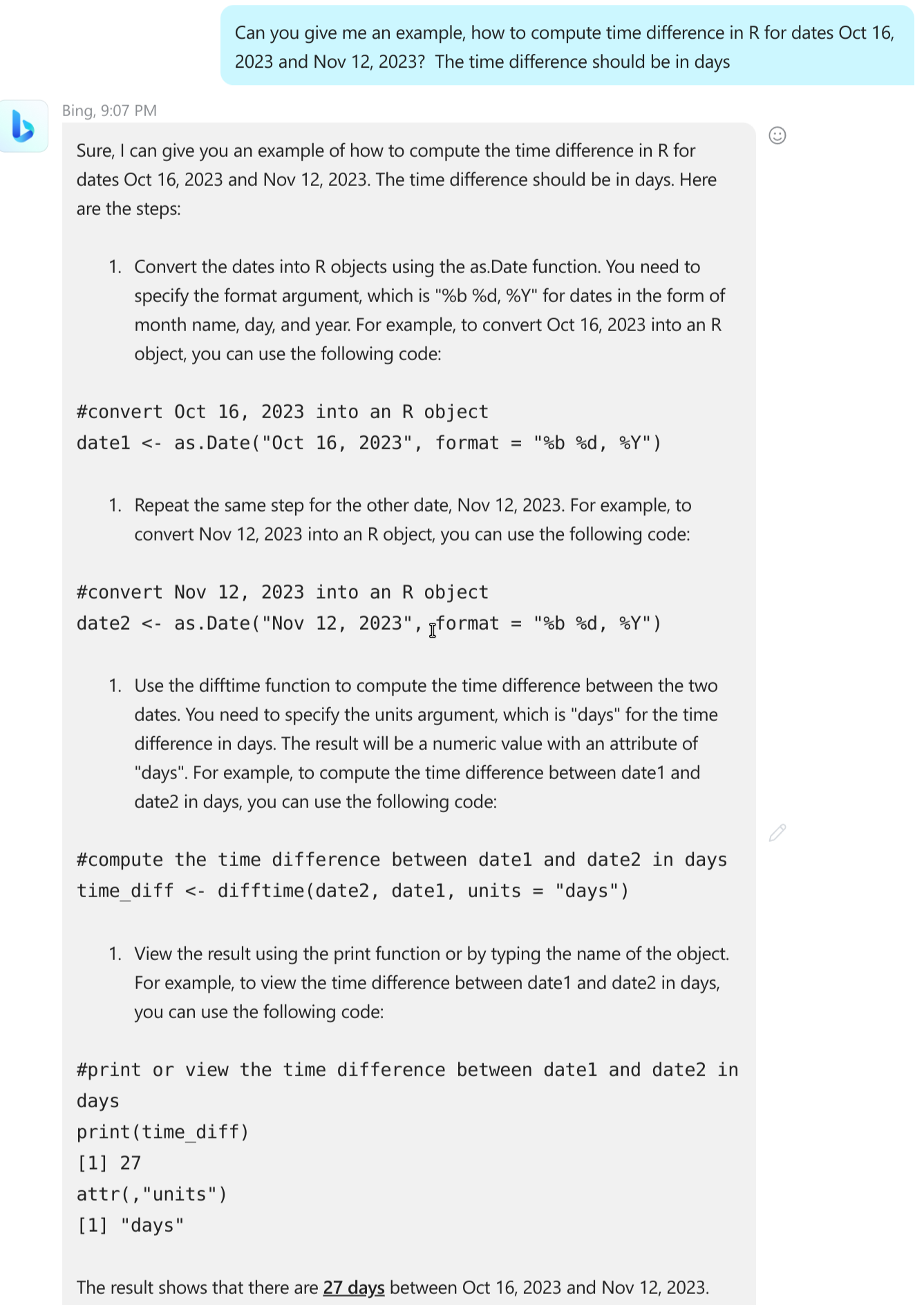
ChatGPT may give very good code examples that only require minimal adjustments.
Novadays AI-based tools are fairly good at doing this. The figure at
right show chatGPT’s answer (incorporated in Bing) to such a
question. This answer is correct and can be incorporated to your code
with only little adjustments. However, one should still look up what do
these functions do and what does format = "%b %d, %Y" mean.
However, the answer my not be enough if you do not know the basics of
R, e.g. what is the assignment operator <- or the comment character
#. Also, it lacks some context and it does not discuss more efficient
or simpler ways to achieve the same task. For instance, it does not
suggest to write the dates in the ISO format YYYY-mm-dd which would
simplify the solution.
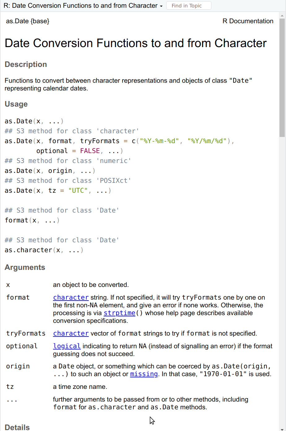
The first page of as.Date help (you can get it with ?as.Date).
The as.Date() help page offers much more information than what
chatGPT gives. In particular, the tryFormats and its default values
are very useful. However, it also assumes more understanding of the
workings of R, e.g. what does the ## S3 method for class 'character'
exactly mean, and which of the functions listed there one actually needs.
So AI-tools are not a substitute to documentation (nor the other way around). AI is great to quickly get a solution. In order to evaluate the solution, you need to know more. But as your time is valuable too–use AI for tasks where you do not need to go in depth, but learn the most important tools in depth.
Here is a simplyfied version of the chatGPT-suggested solution:
dates <- as.Date(c("2023-10-16", "2023-11-12", "2014-07-03"))
                           # ISO dates do not need format specification
difftime(dates[2], dates[1], units="days")
## Time difference of 27 days## Time difference of 3419 daysWhen working with dates, you should also be familiar with lubridate library and tools therein.
K.7.3 Coding style
K.7.3.1 Variable names for election data
One of the decisions you need to make here is how to name the political parties. You definitely do not want to use the full names as those are very long. Here we are actually in a very good situation, as these parties have standard English abbreviation (BJP, INC and YSRCP).
Below is one option:- The original data:
- elections. If there are more election-related things, besides of the dataset, we may call it electionData to stress this is a dataset.
- Corrected original
- electionsFixed
- 2019 only
- elections2019. This assumes we do not need 2019 non-fixed version.
- Sub-datasets for parties.
- electionsBJP
- electionsINC
- electionsYSRCP.
- Winning districts only
- winsBJP
- winsINC
- winsYSRCP
Obviously, there are more options, e.g. if the project is very short, then you may replace elections with just e. If you need more, e.g. also 2024 election data, you may need variable names like elections2019BJP and wins2024INC.
You may also think what to do if the data is about Japan instead, and the party you are interested, 公明党, is abbreviated as 公明. (See Komeito).
K.8 Conditional statements
K.8.1 if-statement
K.8.1.1 Tell if second string longer
This is quite a simple application of if and else:
compareStrings <- function(s1, s2) {
   if(nchar(s2) > nchar(s1)) {
      ## if 2nd string longer the print
      cat("The second string is longer\n")
   }
   ## Do nothing else
}

compareStrings("a", "aa")  # prints
## The second string is longerK.8.1.2 Print if number even
- Here the logic is as follows:
- print the number
- if even, print ” - even”.
for(i in 1:10) {
   cat(i, "\n")  # print the number (and new line)
   if(i %% 2 == 0) {
      cat(" - even\n")  # print 'even' (and new line)
   }
}
## 1
## 2
## - even
## 3
## 4
## - even
## 5
## 6
## - even
## 7
## 8
## - even
## 9
## 10
## - even- Now we need to think more about printing. It goes as follows:
- print the number (no new line)
- if even, print ” - even” (no new line)
- add new line, unconditionally.
for(i in 1:10) {
   cat(i)  # print the number, but do not switch to new line
   if(i %% 2 == 0) {
      cat(" - even")  # print 'even', do not switch to new line
   }
   cat("\n")  # switch to new line at the end of line here
              # whatever number it is
}
## 1
## 2 - even
## 3
## 4 - even
## 5
## 6 - even
## 7
## 8 - even
## 9
## 10 - evenK.8.1.3 Print even/odd
The code is simple, and printing is a bit simpler too
for(i in 1:10) {
   cat(i)  # print the number, but do not switch to new line
   if(i %% 2 == 0) {
      cat(" even\n")  # print 'even' and new line
   } else {
      cat(" odd\n")
   }
}
## 1 odd
## 2 even
## 3 odd
## 4 even
## 5 odd
## 6 even
## 7 odd
## 8 even
## 9 odd
## 10 evenK.8.1.4 Going out with friends
money <- 200
nFriends <- 5
price <- 30
sum <- (nFriends + 1)*price  # friends + myself
total <- sum*1.15  # add tip
if(total > money) {
   cat("Cannot afford 😭\n")
} else {
   cat("Can afford ✌\n")
}
## Cannot afford 😭K.8.1.5 Test porridge temperature
We just need to remove assignments and return():
test_food_temp <- function(temp) {
  if(temp > 120) {
     "This porridge is too hot!"
  } else if(temp < 70) {
     "This porridge is too cold!"
  } else {
     "This porridge is just right!"
  }
}
## The test results are the same:
test_food_temp(119)  # just right!
## [1] "This porridge is just right!"## [1] "This porridge is too cold!"## [1] "This porridge is too hot!"In my opinion, shorter code is easier to read, but different people may have different opinion.
K.8.2 Conditional statements and vectors
K.8.2.1 Should you go to the boba place?
The problem is worded in a somewhat vague manner, so you may need to make it more specific. Here we assume that you only go if you can afford a drink–at least one drink. You do not need that all drinks are affordable.
This means you need to write code that checks if any tea is cheaper than $7.
K.8.2.2 Can you get a drink?
With the original prices:
price <- c(5, 6, 7, 8)
if(any(price <= 7)) {
   cat("You can get a drink\n")
} else {
   cat("This is a too expensive place\n")
}
## You can get a drinkIf they rise the price by $3 across the board then we can just add “3” to the price vector:
price <- price + 3
if(any(price <= 7)) {
   cat("You can get a drink\n")
} else {
   cat("This is a too expensive place\n")
}
## This is a too expensive placeThe results are intuitively obvious–it is affordable using the original prices but not with the new prices.
K.8.2.3 absv() of a vector
The code crashes with a message
## Error in `if (x < 0) ...`:
## ! the condition has length > 1
This is because here the code needs to make two decisions: one for “-3” and another for “3”. But if-else can only handle a single decision!
Note that the decisions for these two values differ–in the first case the code needs to flip the sign, and in the second case the sign must be preserved. But this does not play a role in terms of error messages, the problem here is two decisions, not the fact that the decisions here are different.
K.8.2.4 Step function
The function produces different output, depending on whether \(x \le 0\)
or otherwise. Hence we can use condition x <= 0. From the step
function definition, the true value is 0 and false value 1:
## [1] 0 1 0 1Alternatively, we can use the opposite condition x > 0 and flip the
true and false values:
## [1] 0 1 0 1Obviously, we can also define a function, instead of just using ifelse(),
although here it does not help us much because the code is so short:
## [1] 0 1 0 1K.8.2.5 Leaky relu
As leaky relu needs a different behavior, depending on whether \(x > 0\)
or otherwise, we can use logical condition x > 0. From its
definition, the true
value is just x and the false value is 0.1*x:
## [1] -0.3 3.0 -0.1 1.0K.8.2.6 Sign function
This case is slightly more complex, but we can describe it as two separate cases:- Pick the condition, for instance \(x < 0\).
- now the true value is
-1, but the false value depends on \(x\)
- now the true value is
- In the false case, we have essentially the step function:
- if \(x > 0\), the value is “1”
- otherwise, the value is “0”
Note that we can only get to the “otherwise” if \(x = 0\), because
if \(x < 0\), the first step will already produce. Se we can
write here just
ifelse(x > 0, 1, 0).
Combining these two ifelses, we have
## [1] -1 1 -1 1 0K.8.2.7 Are bowls too hot?
First we can use ifelse() to find if the porridge is too hot or not:
## [1] "all right" "too hot" "all right" "too hot"Next, let’s compose the bowl id message
## [1] "Bowl 1" "Bowl 2" "Bowl 3" "Bowl 4"Now it is just to combine these two messages:
## [1] "Bowl 1 is all right" "Bowl 2 is too hot"   "Bowl 3 is all right"
## [4] "Bowl 4 is too hot"
All this can also be achieved in a shorter form:
## [1] "Bowl 1 is all right" "Bowl 2 is too hot"   "Bowl 3 is all right"
## [4] "Bowl 4 is too hot"
Note that I created the sequence of correct length here using
1:length(temp) instead of hard-coding 1:4 as above.
K.8.3 A few useful and useless tools
K.8.3.1 Are elements in the set?
This is a straightforward application of %in%, all() and any():
vec <- c("a", "b", "c")
set <- c("c", "b", "d")
if(all(vec %in% set)) {
   cat("All in!\n")
} else if(any(vec %in% set)) {
   cat("Some in!\n")
} else {
   cat("None in!\n")
}
## Some in!Note another advantage of %in% over a chain of OR operators: we can
define the set-of-interest in a single place, and use it multiple
times.
K.8.3.2 Southern states
Let’s start by defining the vector of states, and the set of southern states:
states <- c("Madhya Pradesh", "Orissa", "Andra Pradesh",
            "Karnataka", "Gujarat", "Andra Pradesh",
            "Kerala", "West Bengal",
            "Punjab", "Karnataka")
south <- c("Telangana", "Andra Pradesh", "Karnataka",
           "Tamil Nadu", "Kerala", "Puducherry")
Now we can easily test which state is in South:
## [1] FALSE FALSE TRUE TRUE FALSE TRUE TRUE FALSE FALSE TRUEAs creating the corresponding character vector involves a separate
decision for each element of the states vector, we need to use
ifelse():
##  [1] "Not South" "Not South" "South"     "South"     "Not South"
##  [6] "South"     "South"     "Not South" "Not South" "South"
K.8.3.3 x == TRUE versus x
- The condition
x == TRUEcan only be true ifxis of logical type. - If
xis of different type, it will be implicitly converted to logical, if possible. (R cannot automatically convert more complex data types, such as lists.) Number “0” will be converted toFALSE, all other numbers toTRUE. Empty string “” will be converted toFALSE, all other strings toTRUE. - The example code:
## [1] "true"The first expression, x == TRUE results in FALSE, because, well,
x is not TRUE. However, the second if converts x to
logical. This will be TRUE, and hence the message is printed.
So if(x == TRUE) and if(x) are not exactly the same. But it is
a bad practice to write code in a way where x can be of different
type, sometimes logical, sometimes not. Such code is too hard to
understand.
K.9 How R reads files
K.9.1 Accessing files from R
K.9.1.1 R working directory path type
This is absolute path: you see this because “/home/otoomet/tyyq/info201-book” starts with
the root symbol /. See more in Sections 2.3
and 2.4.1.
K.9.1.2 RStudio console working directory
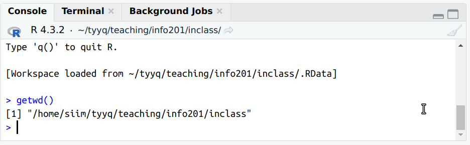
The only way to see it is to run getwd() in rstudio console. You
can run it directly, or you can also execute a line of a script. What
matters is that it runs on console.
The example here shows “/home/siim/tyyq/teaching/info201/inclass” as the current working directory.
K.9.1.3 List files in R and in graphical manager
Assume the current working directory is “/home/siim/tyyq/teaching/info201/inclass” as in the exercise above.
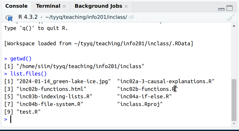
We can use list.files() to see files here.
And here are the same files, seen through the eyes of a graphical file manager (PCManFM). Note the navigation bar above the icons that displays the absolute path of the folder, and the side pane that displays the file system tree (a small view of it only).
It is easy to see that the files are the same. Note that R normally sorts files alphabetically, but file managers may show these in different ways, either alphabetically, by creation time, or you may even manually position individual icons. All this may be configured differently on your computer!
You can also see that here, both R and the file manager show all names in the same way, including the complete extensions like .R or .jpg. This may be different on your computer (and can be changed).
K.10 Markdown and rmarkdown
K.11 Data Frames
K.11.1 What is data frame
K.11.2 Working with data frames
K.11.2.1 Countries and capitals
Appropriate names are country for the country, capital for its capital, and population for the population. We call the data frame as countries (plural) to distinguish it from the individual variable. Obviously, one can come up with other names. We can create the data frame as
countries <- data.frame(
   country = c("Gabon", "Congo", "DR Congo", "Uganda", "Kenya"),
   capital = c("Libreville", "Brazzaville", "Kinshasa", "Kampala", "Nairobi"),
   population = c(2.340, 5.546, 108.408, 45.854, 55.865))
countries
## country capital population
## 1 Gabon Libreville 2.340
## 2 Congo Brazzaville 5.546
## 3 DR Congo Kinshasa 108.408
## 4 Uganda Kampala 45.854
## 5 Kenya Nairobi 55.865where population is in Millions (2022 estimates from Wikipedia).
We can extract the country names by dollar notation as
## [1] "Gabon" "Congo" "DR Congo" "Uganda" "Kenya"and population with double brackets as
## [1] 2.340 5.546 108.408 45.854 55.865Capital using indirect name:
## [1] "Libreville" "Brazzaville" "Kinshasa" "Kampala" "Nairobi"K.11.3 Accessing Data in Data Frames
K.11.3.1 Describe emperors
This is a straightforward application of the functions:
## [1] "name" "born" "throned" "ruled" "died"## [1] 5## [1] 5## name born throned ruled died
## 1 Qin Shi Huang -259 -221 China -210
## 2 Napoleon Bonaparte 1769 1804 France 1821## name born throned ruled died
## 3 Nicholas II 1868 1894 Russia 1918
## 4 Mehmed VI 1861 1918 Ottoman Empire 1926
## 5 Naruhito 1960 2019 Japan NAK.11.3.2 Indirect variable name with dollar notation
R will interpret the workspace variable name that contains the column names as the required column name:
## NULLAs you see, R is looking for a column var. As it cannot find
it, it returns NULL, the special code for empty element.
K.11.3.3 Loop of columns of a data frame
- Column names. No loop needed here:
## [1] "name" "born" "throned" "ruled" "died"- Print names in loop. We can just loop over the names:
## name
## born
## throned
## ruled
## died- Print name and column. We need indirect access here as the column
name is now stored in the variable (called
nbelow). So we can access it asemperors[[n]]:
## name
## [1] "Qin Shi Huang"      "Napoleon Bonaparte" "Nicholas II"
## [4] "Mehmed VI"          "Naruhito"
## born
## [1] -259 1769 1868 1861 1960
## throned
## [1] -221 1804 1894 1918 2019
## ruled
## [1] "China"          "France"         "Russia"         "Ottoman Empire"
## [5] "Japan"
## died
## [1] -210 1821 1918 1926 NA- Print name and type. This is similar to the above, except now we
print
is.numeric(emperors[[n]]).
## name is numeric: FALSE
## born is numeric: TRUE
## throned is numeric: TRUE
## ruled is numeric: FALSE
## died is numeric: TRUE- Print name and minimum. Now use the
TRUE/FALSEfor a logical test, only print average if this is true:
for(n in names(emperors)) {
   cat(n, "")
   if(is.numeric(emperors[[n]])) {
      cat(min(emperors[[n]]))
   }
   cat("\n")
}
## name
## born -259
## throned -221
## ruled
## died NANote: you may want to use min(emperors[[n]], na.rm = TRUE) to avoid
the missing minimum for died column.
K.11.3.4 Emperors who died before 1800
Pure dollar notation is almost exactly the same as the example in the text:
## [1] "Qin Shi Huang" NAWhen using double brackets at the first place, we have
## [1] "Qin Shi Huang" NANote that we have a weird construct here [[...]][..]. It looks
weird, but it perfectly works. emperors[["name"]] is a vector, and
a vector can be indexed using [...].
When we put double brackets in both places, we get
## [1] "Qin Shi Huang" NAThis is perhaps the “heaviest” notation, where it may be hard to keep track of the brackets. However, it is a perfectly valid way to extract emperors!
Finally, NA in the output is related to Naruhito. As we do not know
his year of death, R sends a message that there is one name where we
do not know if he died before 1800. It is a little stupid–as
Naruhito is alive today, he cannot have died before 1800. But we
haven’t explained this knowledge to R.
K.11.3.5 Single-bracket data acess (emperors)
Extract 3rd and 4th row:
##          name born throned          ruled died
## 3 Nicholas II 1868    1894         Russia 1918
## 4   Mehmed VI 1861    1918 Ottoman Empire 1926
All emperors who died in 20th century:
##           name born throned          ruled died
## 3  Nicholas II 1868    1894         Russia 1918
## 4    Mehmed VI 1861    1918 Ottoman Empire 1926
## NA        <NA>   NA      NA           <NA>   NA
This will still give us NA for Naruhito–we haven’t explained to R
in any way that someone who was alive in 2023, cannot have died in
20th century. If a NA is not desired, one can use which():
##          name born throned          ruled died
## 3 Nicholas II 1868    1894         Russia 1918
## 4   Mehmed VI 1861    1918 Ottoman Empire 1926
Name and country of those emperors
##          name          ruled
## 3 Nicholas II         Russia
## 4   Mehmed VI Ottoman Empire
K.11.3.6 Patients aging
First create the data frame:
Name <- c("Ada", "Bob", "Chris", "Diya", "Emma")
Inches <- c(58, 59, 60, 61, 62)
Pounds <- c(120, 120, 150, 150, 160)
age <- c(22, 33, 44, 55, 66)
patients <- data.frame(Name, Inches, Pounds, age)
patients
## Name Inches Pounds age
## 1 Ada 58 120 22
## 2 Bob 59 120 33
## 3 Chris 60 150 44
## 4 Diya 61 150 55
## 5 Emma 62 160 66Adding a single year of age involves just modifying data, but we do not need to filter anythign as this applies to everyone:
##    Name Inches Pounds age
## 1   Ada     58    120  23
## 2   Bob     59    120  34
## 3 Chris     60    150  45
## 4  Diya     61    150  56
## 5  Emma     62    160  67
K.11.4 R built-in datasets
K.11.4.1 co2 data
Let’s take a look at the data:
##         Jan    Feb    Mar    Apr    May    Jun
## 1959 315.42 316.31 316.50 317.56 318.13 318.00
It looks like a numeric vector, but more specifically it is a time
series (“ts”) object, it can be seen with
class():
## [1] "ts"The name suggests that this is some kind of CO2 data. The help page
(can be accessed with ?co2) indicates that this is Mauna Loa
observatory CO2 data, measured as particles per million (ppm),
available for each month from 1959 till 1997.
K.11.5 Learning to know your data
K.11.5.1 CSGO column averages
This can be achieved in a fairly simple fashion by extending the example with for-loop:
csgo <- read_delim("data/csgo-reviews.csv.bz2")
for(col in names(csgo)) {
   if(class(csgo[[col]]) == "numeric") {
      cat(col, ": ", mean(csgo[[col]]), "\n", sep = "")
   }
}
## nHelpful: 620.1343
## nFunny: 6.217729
## nScreenshots: 215.5503
## hours: 805.3682
## nGames: 100.7909
## nReviews: 7.609077Actually, it is better to write the code not as class(x) == "numeric" but as inherits(x, "numeric"). This is because a column
may have multiple classes, and in that case == will give an error.
K.11.5.2 Implausible ice extent/area values
Load data:
## [1] 1062 7Is there any NA-s?
## [1] 0## [1] 0Apparently, all values are valid
The area cannot be negative. The same is true for extent, which is also and area–area of a specific ice concentration. It is harder to come up with a maximum plausible value, but sea ice area cannot exceed the total world sea surface (361M km2 according to wikipedia). Hence the plausible values must be in range \([0, 361]\).
Are all values plausible?
## [1] -9999.00 19.76## [1] -9999.00 15.75All is well with the upper limit–it is much smaller than 361. But some of the values are negative, in particular \(-9999\). This cannot be a valid value and appears to be a way to code missing data.
K.11.5.3 Explore home/destination
We can explore the destinations in a similar fashion as above:
 [1] "St Louis, MO"
 [2] "Montreal, PQ / Chesterville, ON"
 [3] "New York, NY"
 [4] "Hudson, NY"
 [5] "Belfast, NI"
 [6] "Bayside, Queens, NY"
 [7] "Montevideo, Uruguay"
 [8] "Paris, France"
 [9] NA
[10] "Hessle, Yorks"
[11] "Montreal, PQ"
...
The excerpt here shows a number of plausible values, such as “St Luis, MO”. We also see that some values are missing. Unfortunately, there are too many different values,
## [1] 370So that it is very hard to look at all these manually and decide if all are plausible.
If necessary, one can try other options, e.g. to test if the locations contain valid characters only, or even attempt to geo-locate these places with e.g. google maps API.
K.11.5.4 Which value is missing in table()
If you compare the values carefully, you see that NA is missing in the table.
The documentation of table() shows:
?table
...
useNA: whether to include ‘NA’ values in the table.  See ‘Details’.
       Can be abbreviated.
...
This means that you can ask the table to include missings through useNA
argument, e.g.
##
##       1      10      11      12      13   13 15 13 15 B      14      15
##       5      29      25      19      39       2       1      33      37
##   15 16      16       2       3       4       5     5 7     5 9       6
##       1      23      13      26      31      27       2       1      20
##       7       8    8 10       9       A       B       C     C D       D
##      23      23       1      25      11       9      38       2      20
##    <NA>
##     823
"ifany" will show the number of missings, if there are any
missings. Here we have 823 missings.
K.11.5.5 The youngest passenger
As there is a large number of missing age values, you either need to
wrap the results in which():
titanic[which(titanic$age == min(titanic$age, na.rm = TRUE)),
        c("pclass", "survived", "name", "sex", "age")]
## # A tibble: 1 × 5
## pclass survived name sex
## <dbl> <dbl> <chr> <chr>
## 1 3 1 "Dean, Miss. Elizabeth Gladys \"Millvina\"" female
## age
## <dbl>
## 1 0.167or alternatively, use the which.min() function:
## # A tibble: 1 × 5
##   pclass survived name                                        sex
##    <dbl>    <dbl> <chr>                                       <chr>
## 1      3        1 "Dean, Miss. Elizabeth Gladys \"Millvina\"" female
##     age
##   <dbl>
## 1 0.167As there was only a single 2-month old baby, both approaches give the identical result.
K.12 dplyr
K.12.1 Grammar of data manipulation
K.12.1.1 How many trees over size 100?
We can do something like this:
- Take the orange tree dataset
- keep only rows that have size > 100
- pull out the tree number
- find all unique trees
- how many unique trees did you find?
Obviously, you can come up with different lists, e.g. the items 4 and 5 might be combined into one. They are kept separate here that these two items correspond to a single function in base-R.
K.12.1.2 Two ways to find the largest tree
The difference is in how the recipe breaks ties for the largest tree. If there are two largest trees of equal size, these will be put in an arbitrary order. If we pick the first line below, we’ll get one of the largest trees, but not both. The second recipe extracts all trees of maximum size, so it can find all such trees.
In practice, it is more useful not to order the trees and pick the first, but rank them with an explicit way to break ties. For instance
## [1] 1 3 1Will tell that both the first and the third tree are on the “first place”
in descending order. See more with ?rank.
K.12.2 Most important dplyr functions
K.12.2.1 Add decade to babynames
We can compute decade by first integer-dividing year by 10, and then multiplying the result by 10:
## # A tibble: 5 × 6
##    year sex   name         n       prop decade
##   <dbl> <chr> <chr>    <int>      <dbl>  <dbl>
## 1  1987 F     Roshunda    27 0.0000144    1980
## 2  1926 M     Ian         24 0.0000210    1920
## 3  1991 F     Jinna        6 0.00000295   1990
## 4  2008 M     Sepehr       5 0.0000023    2000
## 5  1989 F     Myriam      30 0.0000151    1980
K.12.2.2 How many names over all years
We just need to add the count variable n:
## # A tibble: 1 × 1
##           n
##       <int>
## 1 348120517
K.12.2.3 Shiva for boys/girls
The task list might look like this:- filter to keep only boys (or only girls)
- filter to keep only name “Shiva”
- summarize this dataset by adding up all counts n
There are, obviouly, other options, for instance, you can swapt the filter by sex and filter by name.
## # A tibble: 1 × 1
##   `sum(n)`
##      <int>
## 1      397
## # A tibble: 1 × 1
## `sum(n)`
## <int>
## 1 249K.12.3 Combining dplyr operations
The tasklist for this question (see above) might be:
- Take the orange tree dataset
- keep only rows that have size > 100
- pull out the tree number
- find all unique trees
- how many unique trees did you find?
This can be translated to code as:
## [1] 5So there are 5 different trees.
K.12.4 Grouped operations
K.12.4.1 Titanic fare by class
The computations are pretty much the same as the example in the text:
titanic %>%
   group_by(pclass) %>%
   summarize(avgFare = mean(fare, na.rm=TRUE),
             maxFare = max(fare, na.rm=TRUE),
             avgAge = mean(age, na.rm=TRUE),
             maxAge = max(age, na.rm=TRUE)
             )
## # A tibble: 3 × 5
## pclass avgFare maxFare avgAge maxAge
## <dbl> <dbl> <dbl> <dbl> <dbl>
## 1 1 87.5 512. 39.2 80
## 2 2 21.2 73.5 29.5 70
## 3 3 13.3 69.6 24.8 74The results make sense, as the first class is the most expensive, and the third class the cheapest option. However, it is hard to see why the most expensive 3rd class options was much more than the 2nd class average. It is also reasonable that older people are more likely to travel in upper classes, as they may be wealthier, and their health may be more fragile.
K.12.4.2 Distinct names
- First, the number of distinct names each year. This is exactly the same code as in the example, just without filtering the years down to 2002-2006:
## # A tibble: 10 × 2
##     year     n
##    <dbl> <int>
##  1  1880  1889
##  2  1881  1830
##  3  1882  2012
##  4  1883  1962
##  5  1884  2158
##  6  1885  2139
##  7  1886  2225
##  8  1887  2215
##  9  1888  2454
## 10  1889  2390
The output suggests that the number of distinct names is slowly increasing over time.
- Second, in which years did parents give the largest number of distinct names? Here you can take the previous output, and arrange it by n in the descending order:
babynames %>%
   group_by(year) %>%
   summarize(n = n_distinct(name)) %>%
   arrange(desc(n)) %>%  # most 'productive' years first
   head(5)
## # A tibble: 5 × 2
## year n
## <dbl> <int>
## 1 2008 32510
## 2 2007 32416
## 3 2009 32242
## 4 2006 31624
## 5 2010 31623Apparently, these years are late 2000-s.
K.12.4.3 Most popular boy and girl names
The only difference here is to group by year and sex:
babynames %>%
   filter(between(year, 2002, 2006)) %>%
   group_by(year, sex) %>%
   arrange(desc(n), .by_group = TRUE) %>%
   summarize(name = name[1])
## # A tibble: 10 × 3
## # Groups: year [5]
## year sex name
## <dbl> <chr> <chr>
## 1 2002 F Emily
## 2 2002 M Jacob
## 3 2003 F Emily
## 4 2003 M Jacob
## 5 2004 F Emily
## 6 2004 M Jacob
## 7 2005 F Emily
## 8 2005 M Jacob
## 9 2006 F Emily
## 10 2006 M JacobAs we can see, these are just Emily and Jacob.
K.12.4.4 Three most popular names
The first 3 names in terms of popularity can just be filtered using
the condition rank(desc(n)) <= 3:
## # A tibble: 15 × 5
## # Groups:   year [5]
##     year sex   name        n   prop
##    <dbl> <chr> <chr>   <int>  <dbl>
##  1  2002 M     Jacob   30568 0.0148
##  2  2002 M     Michael 28246 0.0137
##  3  2002 M     Joshua  25986 0.0126
##  4  2003 F     Emily   25688 0.0128
##  5  2003 M     Jacob   29630 0.0141
##  6  2003 M     Michael 27118 0.0129
##  7  2004 F     Emily   25033 0.0124
##  8  2004 M     Jacob   27879 0.0132
##  9  2004 M     Michael 25454 0.0121
## 10  2005 F     Emily   23937 0.0118
## 11  2005 M     Jacob   25830 0.0121
## 12  2005 M     Michael 23812 0.0112
## 13  2006 M     Jacob   24841 0.0113
## 14  2006 M     Michael 22632 0.0103
## 15  2006 M     Joshua  22317 0.0102
As you can see, these are various combinations of “Jacob”, “Michael”, “Joshua” and “Emily”.
K.12.4.5 10 most popular girl names after 2000
This is just about keeping girls only, and arranging by popularity afterward:
babynames %>%
   filter(sex == "F",
          year > 2000) %>%
   group_by(name) %>%
   summarize(n = sum(n)) %>%
   filter(rank(desc(n)) <= 5) %>%
   arrange(desc(n))
## # A tibble: 5 × 2
## name n
## <chr> <int>
## 1 Emma 327254
## 2 Emily 298119
## 3 Olivia 290625
## 4 Isabella 285307
## 5 Sophia 265572We can see that “Emma” has been the most popular.
K.12.4.6 Most popular name by decade
This is noticeably more tricky task:
- First we need to compute decade, this can be done using integer
division
%/%as(year %/% 10)*10. - Thereafter, we need to add all counts n for each name and decade. Hence we group by name and decade, and sum n.
- Thereafter, we need to rank the popularity for each decade. Hence we group again, but now just by decade.
We can do it along these lines:
babynames %>%
   mutate(decade = year %/% 10 * 10) %>%
   group_by(name, decade) %>%
   summarize(n = sum(n)) %>%
   group_by(decade) %>%
   filter(rank(desc(n)) == 1) %>%
   arrange(decade)
## # A tibble: 14 × 3
## # Groups: decade [14]
## name decade n
## <chr> <dbl> <int>
## 1 Mary 1880 92030
## 2 Mary 1890 131630
## 3 Mary 1900 162188
## 4 Mary 1910 480015
## 5 Mary 1920 704177
## 6 Robert 1930 593451
## 7 James 1940 798225
## 8 James 1950 846042
## 9 Michael 1960 836934
## 10 Michael 1970 712722
## 11 Michael 1980 668892
## 12 Michael 1990 464249
## 13 Jacob 2000 274316
## 14 Emma 2010 158715We see that in the early years, “Mary” was leading the pack, later mostly the boy names have dominated.
Note the third line group_by(name, decade). For each decade, this
makes groupings
based on name only, not separately for name and sex. Hence for names
that were given to both boys and girls, we add up all instances across
genders.
K.12.4.7 “Mei” by decade
The final code might look like
babynames %>%
   filter(sex == "F") %>%
   mutate(decade = (year %/% 10) * 10) %>%
   group_by(name, decade) %>%
   summarize(n = sum(n)) %>%  # popularity over all 10 years!
   group_by(decade) %>%
   mutate(k = rank(desc(n))) %>%
   filter(name == "Mei")
## # A tibble: 8 × 4
## # Groups: decade [8]
## name decade n k
## <chr> <dbl> <int> <dbl>
## 1 Mei 1940 18 6274.
## 2 Mei 1950 15 8015
## 3 Mei 1960 36 7082
## 4 Mei 1970 111 5149
## 5 Mei 1980 136 5356.
## 6 Mei 1990 191 5176
## 7 Mei 2000 385 3788.
## 8 Mei 2010 356 3560.We see that “Mei” has gained in popularity over time, starting around 6000th place in popularity in 1940-s down to around 3500 in 2010-s.
A reminder here: the counts n in the table are probably underestimates–names are only included if they are given for at least 5 times.
K.12.5 More advanced dplyr usage
K.12.5.1 Sea and Creek 1980-2000
We can just filter the required years and the required
names, both using
%in%:
## # A tibble: 2 × 5
##    year sex   name      n       prop
##   <dbl> <chr> <chr> <int>      <dbl>
## 1  1985 M     Sea       6 0.00000312
## 2  2000 M     Creek     7 0.00000335
We can see that these names were not popular, but both were given over five times to boys.
K.12.5.2 Name popularity frequency table
Here we want to count how many times are there numbers \(n=5\), \(n=6\), and so on. So we just count it:
## # A tibble: 5 × 2
##       n    nn
##   <int> <int>
## 1   114    16
## 2   355     2
## 3  2023     1
## 4  1195     1
## 5  1153     1
Over all time: we need to aggregate \(n\):
## # A tibble: 5 × 2
##        n    nn
##    <int> <int>
## 1 551485     1
## 2     28   600
## 3 290755     1
## 4  16537     1
## 5   6247     1
K.13 ggplot2
K.13.1 Basic plotting with ggplot2
K.13.2 Most important plot types
K.13.2.1 Age and fare on Titanic
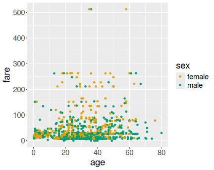
Age versus fare on Titanic
Here we just use age and fare for x and y aesthetics, and sex for the col aesthetics:
Age versus fare on Titanic
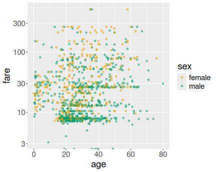
How to make this figure better? I’d probably make the points semi-transparent (see Sections 14.3.2 and 14.3.3) to avoid the massive overplotting. I’d also use log-scale for fare (see Section 14.8.4.1):
Both figures suggest that typically, men paid less and women paid more, also younger passengers were more likely to pay less than older passengers. However, the pattern is quite noisy and there were many elderly and women who chose to travel cheap.
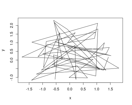
K.13.2.2 COVID-Scandinavia with combined line-point plot
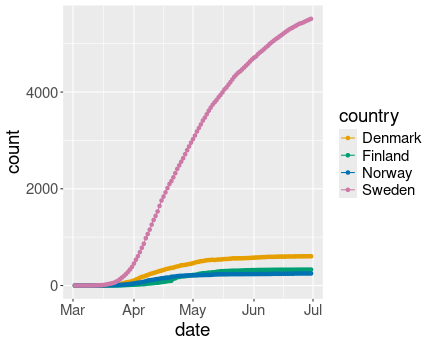
Covid-19 cases in Scandinavia. Combined line-point plot does not look good for densely packed data points.
covS <- read_delim(
   "data/covid-scandinavia.csv.bz2") %>%
   filter(date > "2020-03-01",
          date < "2020-07-01") %>%
   filter(type == "Deaths") %>%
   select(country, date, count)
covS %>%
   ggplot(aes(date, count,
              col = country)) +
   geom_line() +
   geom_point()
Here the result does look less appealing than just the line plot. The reason is that the points are too densely placed. In the Swedish case we can still distinguish points but not see any lines between those, in the other cases all dots overlap, essentially forming thicker lines.
Combined plots are only useful if the data points are sparse. Data is everywhere on these curves, and hence marking the location only makes the result more confusing.
K.13.2.3 Orange tree barplot in different colors
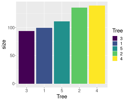
Using aes(..., fill=Tree) uses the values of the data variable
Tree
to
determine the color of the bars.
We can just add the aesthetic fill=Tree to make the bar colors to be
different for diffent trees:
Remember that it is fill aesthetic that controls the fill color, not
the col aesthetic!
But here the colors do not contain any information that is not already embedded in the bars. While colors are usually a nice visual feature, it may be misleading some cases, making the viewer to believe that the colors have a distinct meaning, separate of the bars.
K.13.2.4 Histogram of Titanic data

Here is age histogram:
30 bins seems a good choice here.
Here is age histogram:
A larger number of bins is better here, in order to make more bins available for cheaper tickets, less than 100£, where we have most data.
As you see, age is distributed broadly normally, but fare is more like log-normal with a long right tail of very expensive tickets. Why is it like that? It is broadly related to the fact that human age has pretty hard upper limit, but no such limit exists for wealth. There were very wealthy passengers, but no-one could have been 500 years old.
K.13.2.5 Iris’ petal length distribution
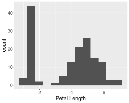
Distribution of petal length in iris data.
The histogram is clearly bimodal:
One group of iris flowers have petals shorter than 2cm, the other group has petals that are about 5cm long.
In my opinion, it does not resemble neither the price nor age histograms–although the age diagram shows a small second peak for children.
The reason for such bimodal distribution can be understood by looking at the petal dimension for individual species:
## # A tibble: 3 × 3
##   Species      min   max
##   <fct>      <dbl> <dbl>
## 1 setosa       1     1.9
## 2 versicolor   3     5.1
## 3 virginica    4.5   6.9
Setosa petals are all less than 2cm long while versicolor a viginica have petals that are at least 3cm long. Hence the bimodal distribution indicates that we have different groups of observations, here different species.
Note also that we can easily differentiate setosa from the two other species, but we cannot easily disentangle versicolor and virginica.
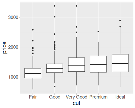
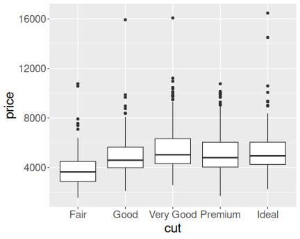
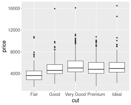
K.13.2.6 Diamond price in a narrow range
Here is the price distribution for mass range \([0.45,0.5]\)ct.

And here for \([0.95,1]\)ct.
Now it is fairly obvious that better cut is associated with higher price.
K.13.2.7 Petal length by species as boxplot

Distribution of petal length of iris species. Boxplot.
We can see that all setosa sepals are shorter than any of versicolor and virginica sepals. This is because the largest setosa outlier (1.9cm), is smaller than any versicolor outlier (3cm). virginica does not have any outliers shown, hence its smallest value is the lower whisker (4.5cm). This is the same message that we got from the exercise above.
In a similar fashion, we see that the upper whisker of versicolor is above the lower whisker of virginica. This means that the longest petals of versicolor are longer than the shortest petals of virginica. Hence we have an overlap.
K.13.2.8 Which plot type?
- Average ticket price is a continuous value while passenger class is a discrete value. Barplot is well suited for this task, but scatterplot and line plot may also work.
- Here you want to display relationship between a continuous distribution (age) and a categorical variable (passenger class). Boxplot is designed for this task, but you may also try density plot, violin plot, and multiple histograms.
K.13.2.9 Fatalities by state
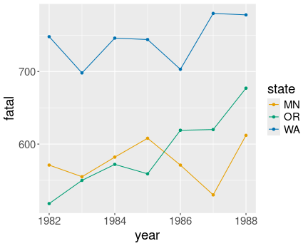
Traffic fatalities over time by state. States are clearly distinct, but the population differences are not visible in any way.
Here we can just make three lines (or line/point combinations) of distinct color–one for each state:
read_delim("data/fatalities.csv") %>%
   ggplot(aes(year, fatal, col = state)) +
   geom_line() +
   geom_point()
We can see that Minnesota and Oregon have comparable numbers of traffic deaths, but there are more fatalities in Washington. However, the figure does not tell whether one state is larger than another one.
K.13.2.10 Covid cases by country
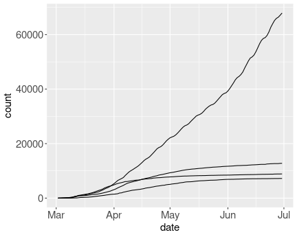
Unsuccessful attempt to do ungrouped line plot.
Here we a) do not specify the col aesthetic, and use group
instead:
## Load and filter data
covS <- read_delim(
   "data/covid-scandinavia.csv.bz2") %>%
   filter(date > "2020-03-01",
          date < "2020-07-01") %>%
   filter(type == "Confirmed") %>%
   select(country, date, count)
## Make the plot
covS %>%
   ggplot(aes(date, count,
              group = country)) +
                           # group is important!!!
   geom_line() +
   theme(text = element_text(size=15))
You may want to label the countries, see Section 14.8.1
K.13.2.11 Point shape to mark the population size
This will just give an error:
read_delim("data/fatalities.csv") %>%
   ggplot(aes(year, fatal,
              shape = pop)) +
                # point shape depends on population
   geom_line() +
   geom_point()
## Error in `geom_line()`:
## ! Problem while computing aesthetics.
## ℹ Error occurred in the 1st layer.
## Caused by error in `scale_f()`:
## ! A continuous variable cannot be mapped to the shape aesthetic.
## ℹ Choose a different aesthetic or use `scale_shape_binned()`.K.13.2.12 Orange tree growth with/without factors
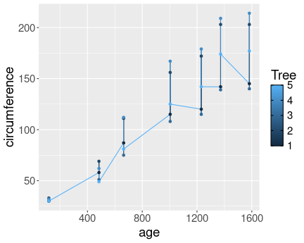
No distinct lines for different trees.
Here is the plot without converting Tree to a factor:
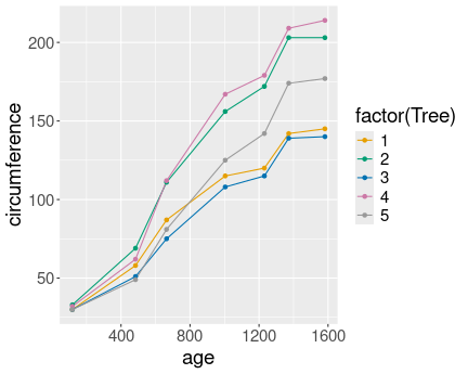
Now the different have distinct lines
And here is the same plot, but now with converting Tree to a factor:
Most importantly, in the first case the different trees are not separated into different lines, as R does not know that the numeric tree id-s are actually discrete values. However, in the second case we tell it, and hence the lines are distinct.
In the first we also have continuous colors (shades of blue), in the second case we have discrete colors.
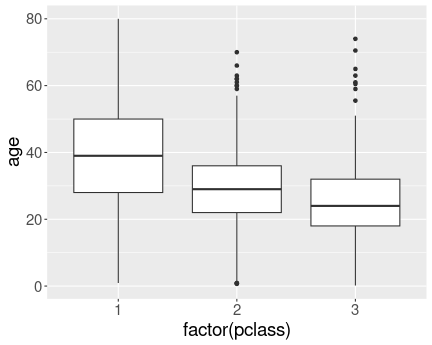
K.13.2.13 Titanic age distribution with/without factors
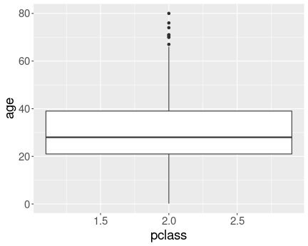
No distinct boxes for different passenger classes.
Here is the plot without converting pclass to a factor:
We have a different box for each class.
And here is the same plot, but now with converting pclass to a factor:
Now we have a separate box for each class. We can see that upper classes are older.
When we attempt to compare the distributions by different values a
continuous variable, then we are in a similar situation as when trying
to split the lines according to a continuous value. ggplot does not
know which continuous values should be grouped together, and hence
does not do any grouping at all. A solution is to convert the
continuous value to a discrete one using factor().
K.13.3 Inheritance
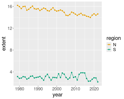
K.13.3.1 Ice extent in January
Everything in color:
ice <- read_delim("data/ice-extent.csv.bz2")
ice %>%
   filter(month == 2) %>%
   ggplot(aes(year, extent, col = region)) +
   geom_line() +
   geom_point()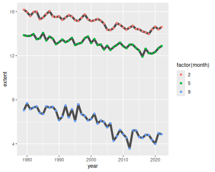
Gray lines:
ice %>%
   filter(month == 2) %>%
   ggplot(aes(year, extent, col = region)) +
   geom_line(aes(group = region),
             col = "gray80",
             linewidth = 2) +
   geom_point()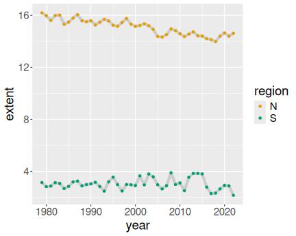
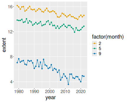
3 Months in north:
ice %>%
   filter(month %in% c(2, 5, 9)) %>%
   filter(region == "N") %>%
   ggplot(aes(year, extent, col = factor(month))) +
   geom_line() +
   geom_point()
3 Months in north, gray lines
ice %>%
   filter(month %in% c(2, 5, 9)) %>%
   filter(region == "N") %>%
   ggplot(aes(year, extent, col = factor(month))) +
   geom_line(aes(group = month),
             col = "gray30",
             linewidth = 2) +
   geom_point()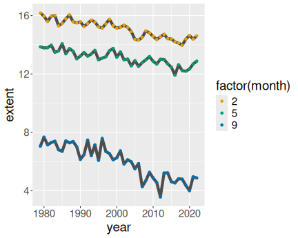
K.13.3.2 Monthly ice extent over years
Here is the code with some explanations. First, load and clean the data:
ice <- read_delim("data/ice-extent.csv.bz2") %>%
   filter(region == "N") %>%
   select(year, month, extent) %>%
   filter(extent > 0)
                           # cleaning
Next, let’s find the first and the last year in the dataset. You are welcome to do it just by analyzing the dataset manually, but here we compute these years. However, there is a problem: we only have a few months for the first and for the last year. Hence, we use instead the first year that contains January data, and the last year the that contains December data. Obviously, you are welcome to choose these years differently:
## What is the first year with January data?
y1 <- ice %>%
   filter(month == 1) %>%
   filter(rank(year) == 1) %>%
   pull(year)
y1  # 1979
## [1] 1979## The last year where we have December data
y2 <- ice %>%
filter(month == 12) %>%
filter(rank(desc(year)) == 1) %>%
pull(year)
y2 # 2012## [1] 2022Below, we’ll create the respective datasets on the fly, by specifying
geom_line(data = filter(ice, year == y1)).
Now let’s compute the decadal averages:
avgExtent <- ice %>%
   mutate(decade = year %/% 10 * 10) %>%
   group_by(decade, month) %>%
   summarize(extent = mean(extent))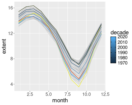
Ice extent on the Northern Hemisphere. Different years, and decadal averages are marked in different colors.
ggplot(ice,
       aes(month, extent)) +
   geom_line(col = "gray77",
                           # all years light gray
             aes(group = year)) +
                           # ensure different lines for different years
   geom_line(data = filter(ice,
                           year == 2012),
                           # 2012 data
             col = "yellow") +
   geom_line(data = filter(ice,
                           year == y2),
             col = "orangered2") +
                           # last year
   geom_line(data = filter(ice,
                           year == y1),
             col = "gold") +
                           # first year
   geom_line(data = avgExtent,
             aes(col = decade,
                 group = decade))
In order to make the plot good, you may need some more fiddling, e.g. you may want to ensure the colors are easy to distinguish, maybe make some lines thicker or semi-transparent, and make the x-scale better. But the information is all here.
K.13.4 Tuning your plots
K.13.4.1 Political parties with one color not specified
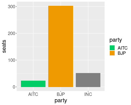
Party which’ color is uncpecified is displayed as gray, more
specifically as value of the argument na.value of the
scale_fill_manual().
Let’s leave out INC and write
data.frame(party = c("BJP", "INC", "AITC"),
seats = c(303, 52, 23)) %>%
ggplot(aes(party, seats, fill=party)) +
geom_col() +
scale_fill_manual(
values = c(BJP="orange2",
AITC="springgreen3")
)As you see, it does not result in an error but a gray bar for INC.
The gray value can be adjusted with na.value, e.g. as
scale_fill_manual(na.value="red").
K.13.4.2 Manually specifying a continuous scale
I do not know how one might be able to manually specify colors for a continuous scale. The problem is that continuous variables can take an infinite number of values–and you cannot specify an infinite number of values manually.
The closest existing option to this is scale_color_gradientn().
This allows you to link a number of data values to specific colors,
and tell ggplot to use gradient for whatever values there are
in-between.
K.13.4.4 March ice extent
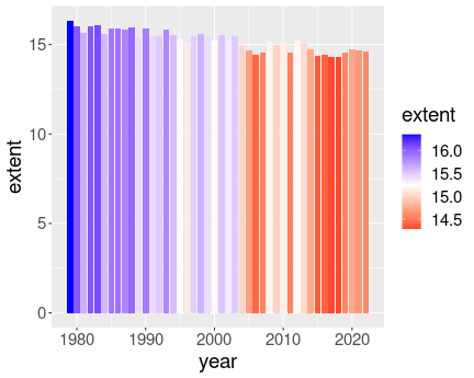
Coloring bars according to the value
ice <- read_delim("data/ice-extent.csv.bz2")
## create a separate filtered df--
## we need it for both plotting
## and for computing the average
ice3 <- ice %>%
filter(month == 3,
region == "N")
avg <- ice3$extent %>%
mean()
ggplot(ice3,
aes(year, extent, fill = extent)) +
geom_col() +
scale_fill_gradient2(low = "red",
mid = "white",
high = "blue",
midpoint = avg)Here one might want to make plot not of the extent, but of the difference between the extent and it’s average (baseline) value.
K.13.4.5 Adjust text labels
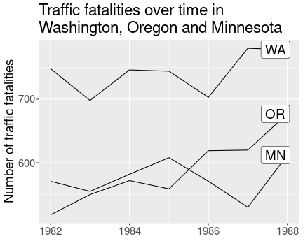
Here is an example solution:
fts <- read_delim("data/fatalities.csv")
ftsLast <- fts %>%
group_by(state) %>%
filter(rank(desc(year)) == 1)
ggplot(fts,
aes(year, fatal,
group = state)) +
geom_line() +
geom_label(data = ftsLast,
aes(label = state),
nudge_x = -0.3) +
labs(
y = "Number of traffic fatalities",
title = "Traffic fatalities over time in
Washington, Oregon and Minnesota") +
theme(axis.title.x = element_blank())It moves the plot labels slightly left (nudge_x = -0.3) and removes
the year label by using theme(). It also demonstrates the usage
of multi-line strings for title.
K.13.4.6 Line-text-plot
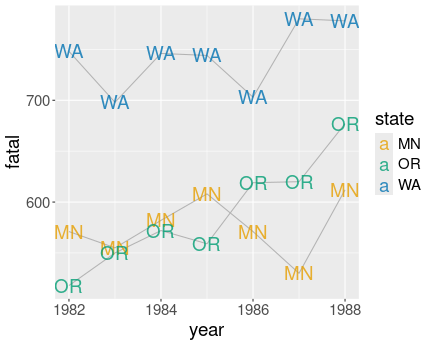
Here is an example solution:
ggplot(fts,
aes(year, fatal,
group = state)) +
geom_line(col = "gray70") +
geom_text(aes(label = state,
col = state),
alpha = 0.8)I did the lines light gray (gray70), and labels for different states
have different color. I also made the label somewhat transparent
(alpha = 0.8) to reduce the problem of overlapping.
However, the figure is not great. Most importantly, labeling the points with exactly the same labels while also connecting these with lines seems unnecessary, and noisy. One label would be sufficient here.
Also, the “MN” and “OR” labels are partly overlapping, this is not visually pleasant. ggrepel package might help here.
Finally, the color key is completely unnecessary–the labels already
convey the exact information. It
can removed easily by + guides(col = "none").
K.13.4.7 Diamonds with log scale
Here and example with both x and y in log: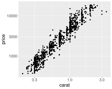
Diamond weight-price plot in log scale. The dense region of small weight and price values is now clearly visible.
diamonds %>%
sample_n(1000) %>%
ggplot(aes(carat, price)) +
geom_point() +
scale_x_log10() +
scale_y_log10()As you can see, the graph is now fairly evenly populated with dots (diamonds). The relationship also looks remarkably linear.
Which graph is the best is debatable. The log-log plot here clearly solves the oversaturate lower-left corner problem in the original image, and the linear relationship looks appealing. However, humans are not that good at understanding log scales. The relationship is is curved in the linear scale–larger diamonds are not just more expensive, but the value of extra carat increases with weight. This fact is not obvious from the log-log scale figure.
The two log-linear relationship are not that useful in my opinion.
K.13.4.8 Arctic Death Spiral
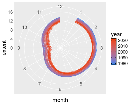
The path of northern polar sea ice through the years.
ice <- read_delim(
"data/ice-extent.csv.bz2") %>%
filter(extent > 0,
region == "N") %>%
select(year, month, extent)
ggplot(ice,
aes(month, extent,
col = year,
group = year)) +
geom_line(linewdith = 0.3) +
coord_polar() +
scale_color_gradient(
low = "dodgerblue2",
high = "orangered2") +
scale_y_continuous(limits = c(0, NA)) +
scale_x_continuous(breaks = 1:12,
limits = c(0,12))I keep year continuous, as otherwise the plot would contain too many discrete colors for years. However, I need to group the lines by year, otherwise ggplot would just show a single line.
Some works should be done with breaks and limits: I tell ggplot to set
the center of the plot to be 0 and leave the outer limit for it to be
figure out (scale_y_continuous(limits = c(0, NA))). I tell that I
want to mark months 1 to 12 (breaks = 1:12), but the angle should
start with month 0 (limits = c(0, 12)). Otherwise December and
January will overlap.
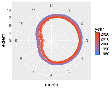
The “Death Spiral of Arctic” with December connected to the following January.
## data for 'month0'
month0 <- ice %>%
filter(month == 12) %>%
# take December data
mutate(month = 0,
# set month = 0
year = year + 1)
# ...it is for next year
rbind(ice, month0) %>%
# merge month 0 to data
ggplot(aes(month, extent,
col = year,
group = year)) +
geom_line(linewdith = 0.3) +
coord_polar() +
scale_color_gradient(
low = "dodgerblue2",
high = "orangered2") +
scale_y_continuous(limits = c(0, NA)) +
scale_x_continuous(breaks = 1:12,
limits = c(0,12))The month-0 data is created by just picking the December data, and
thereafter manually setting the month to 0 and year to the following
year. Thereafter, month-0 is merged with the ice data frame using
rbind() (See section 15.1.1). The plotting code
is exactly the same as above.
K.13.5 More geoms and plot types
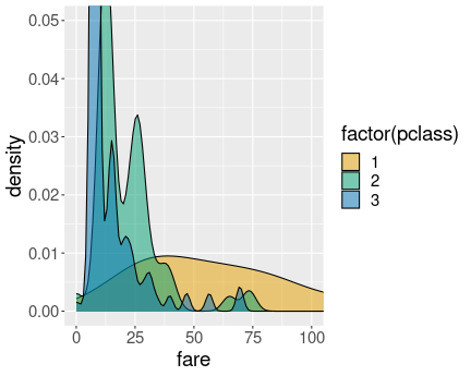
K.13.5.2 Colored violinplot
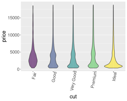
Price distribution by cut. Violinplot.
The solution is just to add fill = cut to the aes() function. I
have also added alpha = 0.6 as I like the transparent colors.
ggplot(diamonds,
aes(cut, price,
fill = cut)) +
geom_violin(alpha = 0.6) +
theme(axis.text.x =
element_text(angle=80,
hjust = 0.9)) +
guides(fill = "none")theme(...) rotates the x-axis labels, and guides(...) removes
the redundant color key.
K.13.5.3 All years on ice extent-area plot
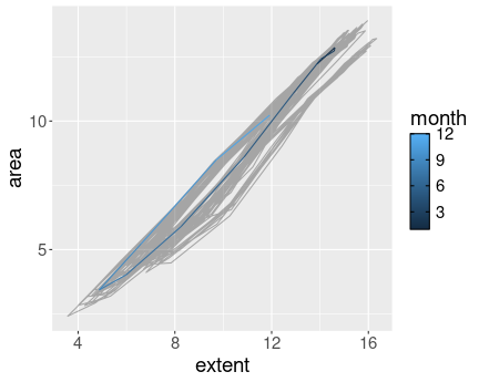
Ice extent versus area. All years marked in gray, 2022 in blue.
Here is a solution. The main trick is to use data inheritance and to plot first all years in gray, and thereafter the selected ones with a custom color:
ice <- read.delim(
"data/ice-extent.csv.bz2") %>%
filter(extent > 0, area > 0) %>%
# clean
filter(region == "N") %>%
# only northern hemisphere
arrange(year, month)
# ensure in temporal order
ggplot(ice, aes(extent, area)) +
geom_path(alpha = 0.3) +
# semi-transparent
geom_path(data = filter(ice,
year == 2022),
aes(col = month))We may want to give the plot better labels, and maybe mark a few more years.
If you want to display more than one year on this graph, then it may
be better to display years using different colors, and label months
with numbers on the graph (using geom_text() or similar).
K.13.5.4 All diamonds with different methods
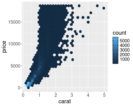
2D histogram with hexagonal bins
First the hexagonal bins:
(Note that you need to install hexbin package for geom_hexbin() to work.)
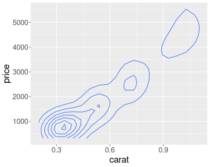
Density plot (contour plot) of distribution of diamonds
And now the density plot:
Note that by default, the density plot only covers the most dense area of the diamonds’ distribution.
As you can see, the hexagonal histogram looks more beautiful, but density contours are clearer to read. Personally, I prefer colored versions for presentations, but the lines are easier to read to understand the details.
K.13.5.5 Cut versus price
There are, obviously, many ways to display the relationship. Here is the best that I was able to come up with: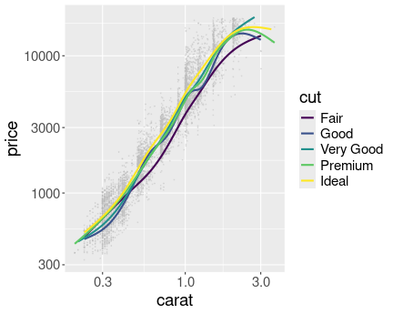
The relationship between diamonds’ weight and price, by different cut.
diamonds %>%
sample_n(6000) %>%
ggplot(aes(carat, price,
col = cut)) +
geom_point(col = "gray",
size = 0.3,
alpha = 0.3) +
geom_smooth(se = FALSE) +
scale_x_log10() +
scale_y_log10()I find the points too noisy, hence I plot a subset of them small and transparent, and in gray. Instead, I use color-coded scatterplot smoothers to indicate the average price by cut. Finally, log scale ensures that the densest part of the distribution, the one at low carat and price, is clearly visible.
As you can see, “fair” cut clearly commands inferior price, but for most other cuts, the price difference is very small.
K.14 More about data manipulations
K.14.1 Merging data
K.14.1.1 Use cbind() to merge students
Here is the example code:
students <- data.frame(
name = c("Cecilia", "Marco", "Guangqi"),
"GPA 2023-au" = c(4.0, 3.8, 2.8),
check.names = FALSE)
students24 <- data.frame(
name = c("Marco", "Cecilia", "Guangqi"),
"gpa 2024-wi" = c(3.7, 3.9, 3.0),
check.names = FALSE)
cbind(students, students24)## name GPA 2023-au name gpa 2024-wi
## 1 Cecilia 4.0 Marco 3.7
## 2 Marco 3.8 Cecilia 3.9
## 3 Guangqi 2.8 Guangqi 3.0Hence cbind() will include two copies of the name column.
This is because cbind() just “solders” the two data frames into one,
line-by-line. That is all it does. merge(), however, knows that
name is the key–the unique identifier of students. And hence it
knows that there is no need to repeat the same identifier twice.
K.14.1.2 Column names do not match
First, let’s create the tables:
gpa <- data.frame(student = c("Cecilia", "Marco"),
gpa = c(4.0, 3.8))
students <- data.frame(name = c("Cecilia", "Marco"),
student = c(2023, 2024))Now the answers:
You need to use
by.xandby.yto tellmerge()how are the specific keys called in each table:## student gpa student.y ## 1 Cecilia 4.0 2023 ## 2 Marco 3.8 2024As you see above, the other “student” column will be renamed to
student.y. You can rename it afterward if you wish, check also out thesuffixesargument formerge().If you merge both tables without specifying the key you’ll get
## [1] student gpa name ## <0 rows> (or 0-length row.names)– a data frame with no rows. This is because by default it picks the key as the column(s) that are common in both tables. Here this is “student”. Now there are no values in student columns that match across the tables, so it thinks that there are no common cases, and as we do not require to keep all rows in either table (it will perform inner join by default), it just drops everything.
K.14.1.3 Keeping and not keeping non-matches
- In this case you want to keep all relevant calls, but only those towers that match with these calls. These towers tell where the calls took place, the location of other towers is irrelevant.
- This is a sort of the opposite task. You want to filter the relevant towers, those that are located in the regions of interest. If you merge the datasets, you want to keep all these towers, but only those calls that take place there. The other calls take place elsewhere and hence they are irrelevant.
- Here you want to keep only those students where you have both a) email address; and b) major. While there may be math majors with no valid email address recorded, such cases do not help you anywhere in terms of the mailing list. You may include students with missing majors in your mailing list, but those are most likely not math majors, so you probably do not want to do it. Hence you will likely drop both missing majors and missing emails.
K.14.1.4 Customers and orders
- Merge key is the customer id, labeled “id” in the customer table and “customer” in the orders’ table.
- This is not quite clear. I am perhaps inclined only to keep these rows where the keys match, otherwise I am not able to tell who is the most valuable customer. But you can also argue that we should keep all orders, just to alert the boss if there is a valuable customers whose name (and age) we do not know.
- The combined data will contain 6 rows, all the orders of known customers (all, except the 7th row by customer #107).
- The answers:
customersOrders <- merge(customers, orders,
all = FALSE, # only keep rows that match
by.x = "id", by.y = "customer")
customersOrders # just view to see what did you get## id name age id.y amount
## 1 101 Jay 20 1001 25
## 2 101 Jay 20 1005 70
## 3 102 Bhagavad 30 1006 75
## 4 103 Arjuna 40 1002 52
## 5 103 Arjuna 40 1003 120
## 6 103 Arjuna 40 1004 170 # note: 'id' from 'orders' is renamed to
# to 'id.y'
## the total most valuable customer
customersOrders %>%
group_by(name) %>% # for each customer
summarize(total = sum(amount)) %>%
arrange(desc(total))## # A tibble: 3 × 2
## name total
## <chr> <dbl>
## 1 Arjuna 342
## 2 Jay 95
## 3 Bhagavad 75So the most valuable customer is Arjuna who spent $342 in total.
## most valuable young customer
customersOrders %>%
filter(age < 35) %>%
group_by(name) %>% # for each customer
summarize(total = sum(amount)) %>%
arrange(desc(total))## # A tibble: 2 × 2
## name total
## <chr> <dbl>
## 1 Jay 95
## 2 Bhagavad 75So the most valuable young customer is Jay ($95)
## Total amount by Bhagavad
customersOrders %>%
filter(name == "Bhagavad") %>%
pull(amount) %>%
sum()## [1] 75Bhagavad spent $75 in total.
Note that we chose to ignore unknown customer #107. We could have preserved all orders instead, then it would have shown up with a missing name.
K.14.2 Dimension of cross-join
It is easy to see that the result has nrow(df1)*nrow(df2) = 4000
rows and ncol(df1) + ncol(df2) = 37 columns. This is because each
40 rows of df1 will be “multiplied” by each 100 rows of df2, their
columns are simply combined together.
As this example suggests, cross-join can easily lead to huge tables.
K.14.3 Create grid
This is just basic many-to-many merge:
dfx <- data.frame(x = seq(0, 1, length.out = 5))
dfy <- data.frame(y = seq(0, 1, length.out = 5))
merge(dfx, dfy)## x y
## 1 0.00 0.00
## 2 0.25 0.00
## 3 0.50 0.00
## 4 0.75 0.00
## 5 1.00 0.00
## 6 0.00 0.25
## 7 0.25 0.25
## 8 0.50 0.25
## 9 0.75 0.25
## 10 1.00 0.25
## 11 0.00 0.50
## 12 0.25 0.50
## 13 0.50 0.50
## 14 0.75 0.50
## 15 1.00 0.50
## 16 0.00 0.75
## 17 0.25 0.75
## 18 0.50 0.75
## 19 0.75 0.75
## 20 1.00 0.75
## 21 0.00 1.00
## 22 0.25 1.00
## 23 0.50 1.00
## 24 0.75 1.00
## 25 1.00 1.00See also the function expand.grid().
K.14.4 Reshaping
K.14.4.1 Alcohol disorders wide form
Instead of grouping the values by country, you can group them by sex. So sex will be in rows and countries in columns. The result might look like
| sex | Argentina | Kenya | Taiwan | Ukraine | United States |
|---|---|---|---|---|---|
| M | 3.069886 | 0.7469638 | 0.8912813 | 3.895495 | 2.927539 |
| F | 1.170313 | 0.6539660 | 0.2611961 | 1.425379 | 1.729168 |
We have essentially rotated the data by 90°. This table is also easy to understand. In terms of Section 15.2.1, we use table (b) instead of (a).
K.14.4.2 Alcohol disorder data in pure wide form
If we do not have countries in separate rows, then we need more columns. Currently we have two sexes for each state. We still need those two, but now they must be in the same row for every country. So we’ll have a peculiar data frame with a single row only! So the resulting dataset will contain a single row and a large number of columns, one for each country-state combination. There will be no distinct “country” column nor a separate “sex”. It might look like
| MArgentina | MKenya | MTaiwan | MUkraine | MUnited States | FArgentina | FKenya | FTaiwan | FUkraine | FUnited States |
|---|---|---|---|---|---|---|---|---|---|
| 3.069886 | 0.7469638 | 0.8912813 | 3.895495 | 2.927539 | 1.170313 | 0.653966 | 0.2611961 | 1.425379 | 1.729168 |
Note that we now need to add country name to the column names to make clear which “M” means Argentina and which one Taiwan.
K.14.4.3 Reshape patients data
This data frame is in a wide form as there are two columns, male and female, that contain counts. The NA is somewhat misleading, it would be more appropriate to put “0” in that place instead.
Hence we can reshape it into a long form:
patients <- data.frame(pregnant = c("yes", "no"),
male = c(NA, 25),
female = c(11, 20))
patients %>%
pivot_longer(!pregnant,
names_to = "sex",
values_to = "count")## # A tibble: 4 × 3
## pregnant sex count
## <chr> <chr> <dbl>
## 1 yes male NA
## 2 yes female 11
## 3 no male 25
## 4 no female 20The result has three columns-pregnant, sex and count. We may want remove the NA-row.
K.14.4.4 Alcohol disorders with sexes in rows
First the long form with better sex names:
longDisorders <- disorders %>%
pivot_longer(!country,
values_to = "disorders",
names_to = "sex") %>%
mutate(sex = gsub("disorders", "", sex))
longDisorders## # A tibble: 10 × 3
## country sex disorders
## <chr> <chr> <dbl>
## 1 Argentina M 3.07
## 2 Argentina F 1.17
## 3 Kenya M 0.747
## 4 Kenya F 0.654
## 5 Taiwan M 0.891
## 6 Taiwan F 0.261
## 7 Ukraine M 3.90
## 8 Ukraine F 1.43
## 9 United States M 2.93
## 10 United States F 1.73And now reshape it to the alternate wide form:
## # A tibble: 2 × 6
## sex Argentina Kenya Taiwan Ukraine `United States`
## <chr> <dbl> <dbl> <dbl> <dbl> <dbl>
## 1 M 3.07 0.747 0.891 3.90 2.93
## 2 F 1.17 0.654 0.261 1.43 1.73As we want to put countries in columns, we need to use names_from = "country".
K.14.4.5 Alcohol disorders widest possible
First the long form (with shorter sex names), exactly as above:
longDisorders <- disorders %>%
pivot_longer(!country,
values_to = "disorders",
names_to = "sex") %>%
mutate(sex = gsub("disorders", "", sex))Here the groups are in two columns: country and sex. We want both
of these to be in columns, hence we need names_from = c(country, sex). There is only a single column of disorder values, so
values_from = disorders will stay the same:
## # A tibble: 1 × 10
## Argentina_M Argentina_F Kenya_M Kenya_F Taiwan_M Taiwan_F Ukraine_M
## <dbl> <dbl> <dbl> <dbl> <dbl> <dbl> <dbl>
## 1 3.07 1.17 0.747 0.654 0.891 0.261 3.90
## Ukraine_F `United States_M` `United States_F`
## <dbl> <dbl> <dbl>
## 1 1.43 2.93 1.73When reshaping it directly, without transforming to the long form first, we have one grouping column, country. Hence we need
## # A tibble: 1 × 10
## disordersM_Argentina disordersM_Kenya disordersM_Taiwan
## <dbl> <dbl> <dbl>
## 1 3.07 0.747 0.891
## disordersM_Ukraine `disordersM_United States` disordersF_Argentina
## <dbl> <dbl> <dbl>
## 1 3.90 2.93 1.17
## disordersF_Kenya disordersF_Taiwan disordersF_Ukraine
## <dbl> <dbl> <dbl>
## 1 0.654 0.261 1.43
## `disordersF_United States`
## <dbl>
## 1 1.73K.14.4.6 Different ways to represent location-altitude-time data
It is fairly easy to see that there are 8 options to present these data as a data frame. Namely, the data have 3 groupings: location, altitude, and time. Each of these grouping can be either in rows, or columns, independently of each others. So there are 2 possibilities for each grouping, and hence \(2\times2\times2 = 8\) in total.
What are missing from the example tables are- Loc, Alt in columns; Time in rows
- Loc, Time in columns; Alt in rows
- Loc in columns; Time, Alt in rows
K.14.4.7 Ice extent data grouping dimensions
As a refresher, the ice extent data looks like
ice <- read.delim(
"data/ice-extent.csv.bz2") %>%
filter(extent > 0, area > 0) %>%
# clean
select(year, month, region, extent, area)
ice %>%
head(3)## year month region extent area
## 1 1978 11 N 11.65 9.04
## 2 1978 11 S 15.90 11.69
## 3 1978 12 N 13.67 10.90The grouping dimensions: it is a bit tricky. One of these is region (North and South). The other one can be time (year-month combination), or you can talk about two other dimensions: year and month. In my opinion, it makes more sense to consider a linear time (year-month combination) as a single dimensions. But if you want to compare the same month across different years, it may make more sense to talk about two dimensions, year and month.
In terms of the region, the dataset is in long form. There is only a single column region that contains region type (“N” and “S”).
Values are extent and area. And yes, the differ by year and month.
Should these be combined together into an additional grouping dimension? Maybe. Unlike the example of temperature and humidity, they are measured in the same physical units (million km2 in these data), they have fairly similar values, and hence they can be represented on the same graph. But computing averages or filtering may still not make sense. Personally, I’d keep them separate.
We need to combine the month name and value column name. For instance, area2 for area in February and extent11 for November extent.
K.14.4.8 Groupings for COVID Scandinavia data
This dataset contains 2 or 3 groupings: country and date are grouping dimensions for sure, type may be counted as such
These data are in the long form: one row is a combination of country-date-type, no single grouping is gathered into one line.
Personally, I would not count type (= Confirmed/Deaths) as groupings, as these are quite different measures. But technically, it can be counted as grouping.
But I cannot imagine what you can do with the count column without filtering out either deaths or confirmed cases.
I see 3 values in the current form: count (a number), lockdown (a date), and population (a number). If we treat type not as grouping dimension, then instead of count we have two columns: Confirmed and Deaths, in that case we have 4 values.
Only confirmed and death counts change along country and date. Population and lockdown are different for different countries, but do not change over time.
code2 is just another name for the country (its 2-letter iso code). It is equivalent to country column and contains no independent information. So if you want to preserve it, then it should be handled exactly the same way as country. So if you convert it into a row where each row is a country, you want to add a column “code2” to that row. If you want to put countries in columns, then you probably want to remove code2 alltogether. Or maybe combine it into a column name like deaths_denmark_DK, admittedly somewhat clunky and redundant.
K.14.4.9 Alcohol disorders with countries in columns
First let’s get the data into long for again:
disorders <- read_delim("data/alcohol-disorders.csv")
disordersL <- disorders %>%
pivot_longer(c(disordersM, disordersF),
values_to = "disorders",
names_to = "sex") %>%
mutate(sex = ifelse(sex == "disordersF", "F", "M"))
disordersL %>%
sample_n(4)## # A tibble: 4 × 6
## country Code Year population sex disorders
## <chr> <chr> <dbl> <dbl> <chr> <dbl>
## 1 Kenya KEN 2019 50951452 M 0.773
## 2 Ukraine UKR 2017 44657260 M 3.58
## 3 Taiwan TWN 2015 23512136 F 0.261
## 4 Kenya KEN 2018 49953300 M 0.752Next, we need to tell to pivot_wider() that names should be taken
from both country and iso2 while the values are population and
disorders:
disordersL %>%
pivot_wider(names_from = c(country, Code),
values_from = c(population, disorders)) %>%
sample_n(3)## # A tibble: 3 × 12
## Year sex population_Argentina_ARG population_Kenya_KEN
## <dbl> <chr> <dbl> <dbl>
## 1 2017 M 44054616 48948140
## 2 2015 F 43257064 46851496
## 3 2017 F 44054616 48948140
## population_Taiwan_TWN population_Ukraine_UKR
## <dbl> <dbl>
## 1 23665028 44657260
## 2 23512136 44982568
## 3 23665028 44657260
## `population_United States_USA` disorders_Argentina_ARG
## <dbl> <dbl>
## 1 329791232 3.02
## 2 324607776 1.17
## 3 329791232 1.16
## disorders_Kenya_KEN disorders_Taiwan_TWN disorders_Ukraine_UKR
## <dbl> <dbl> <dbl>
## 1 0.742 0.886 3.58
## 2 0.654 0.261 1.43
## 3 0.658 0.260 1.29
## `disorders_United States_USA`
## <dbl>
## 1 2.88
## 2 1.73
## 3 1.72Why do we need to take names from both country and iso2 columns, resulting in awkward column names like disorders_Kenya_Ken? Because if you leave one of these, e.g. iso2, out then it is considered to be a grouping column, similar to year or sex. Hence computer tries assumes the country codes are groupings, and attempts to assign each value of the group to each country. This will result in a lot of NA-s:
disordersL %>%
pivot_wider(names_from = c(country),
values_from = c(population, disorders)) %>%
sample_n(3)## # A tibble: 3 × 13
## Code Year sex population_Argentina population_Kenya
## <chr> <dbl> <chr> <dbl> <dbl>
## 1 USA 2015 M NA NA
## 2 KEN 2016 M NA 47894668
## 3 ARG 2017 M 44054616 NA
## population_Taiwan population_Ukraine `population_United States`
## <dbl> <dbl> <dbl>
## 1 NA NA 324607776
## 2 NA NA NA
## 3 NA NA NA
## disorders_Argentina disorders_Kenya disorders_Taiwan disorders_Ukraine
## <dbl> <dbl> <dbl> <dbl>
## 1 NA NA NA NA
## 2 NA 0.744 NA NA
## 3 3.02 NA NA NA
## `disorders_United States`
## <dbl>
## 1 2.93
## 2 NA
## 3 NAIn case of country and Code, I’d probably just remove country, as Code carries the same information and will make the relevant column names more clear:
disordersL %>%
select(!country) %>%
pivot_wider(names_from = c(Code),
values_from = c(population, disorders)) %>%
sample_n(3)## # A tibble: 3 × 12
## Year sex population_ARG population_KEN population_TWN population_UKR
## <dbl> <chr> <dbl> <dbl> <dbl> <dbl>
## 1 2018 M 44413592 49953300 23726186 44446952
## 2 2015 M 43257064 46851496 23512136 44982568
## 3 2017 F 44054616 48948140 23665028 44657260
## population_USA disorders_ARG disorders_KEN disorders_TWN disorders_UKR
## <dbl> <dbl> <dbl> <dbl> <dbl>
## 1 332140032 3.04 0.752 0.892 3.53
## 2 324607776 3.07 0.747 0.891 3.90
## 3 329791232 1.16 0.658 0.260 1.29
## disorders_USA
## <dbl>
## 1 2.89
## 2 2.93
## 3 1.72K.14.4.10 Reshape ice extent
reshape the data to a wide form:
## # A tibble: 4 × 26 ## year region area_11 area_12 area_1 area_2 area_3 area_4 area_5 area_6 ## <int> <chr> <dbl> <dbl> <dbl> <dbl> <dbl> <dbl> <dbl> <dbl> ## 1 1978 N 9.04 10.9 NA NA NA NA NA NA ## 2 1978 S 11.7 6.97 NA NA NA NA NA NA ## 3 1979 N 8.37 10.6 12.4 13.2 13.2 12.5 11.1 9.34 ## 4 1979 S 11.3 6.24 3.47 2.11 2.66 5.45 8.3 11.2 ## area_7 area_8 area_9 area_10 extent_11 extent_12 extent_1 extent_2 ## <dbl> <dbl> <dbl> <dbl> <dbl> <dbl> <dbl> <dbl> ## 1 NA NA NA NA 11.6 13.7 NA NA ## 2 NA NA NA NA 15.9 10.4 NA NA ## 3 6.69 5.06 4.58 6.19 10.9 13.3 15.4 16.2 ## 4 13.3 13.8 14.3 13.7 15.3 9.24 5.4 3.14 ## extent_3 extent_4 extent_5 extent_6 extent_7 extent_8 extent_9 ## <dbl> <dbl> <dbl> <dbl> <dbl> <dbl> <dbl> ## 1 NA NA NA NA NA NA NA ## 2 NA NA NA NA NA NA NA ## 3 16.3 15.4 13.9 12.5 10.3 8.04 7.05 ## 4 4 7.49 10.8 14.2 16.5 17.7 18.2 ## extent_10 ## <dbl> ## 1 NA ## 2 NA ## 3 8.75 ## 4 17.8As you see, by default the variables names are extent_12 and so. The default, alphabetic order is not the best one, you may want to convert the month names into a 2-digit form so January would be “01” and so in order to ensure that the alphabetic order corresponds to the logical order. You can also see that Year-month combinations that are missing in the dataset are replaced by NA.
wide by region:
## # A tibble: 4 × 6 ## year month area_N area_S extent_N extent_S ## <int> <int> <dbl> <dbl> <dbl> <dbl> ## 1 1978 11 9.04 11.7 11.6 15.9 ## 2 1978 12 10.9 6.97 13.7 10.4 ## 3 1979 1 12.4 3.47 15.4 5.4 ## 4 1979 2 13.2 2.11 16.2 3.14This dataset contains 4 value columns only and is easier to grasp.
K.14.4.11 Ice extent and area over time
First, calculate the average area and extent by year. This can be done by justgroup_by(), see Section 13.5.
Now, the plot. ggplot is designed in a way that it is easier to plot a single
column (call it Mkm2), and split it into two lines of different
color by another column (call it type). However, in these data we
have separate columns for area and extent. So we want to transform it
into a long form according to these measures:
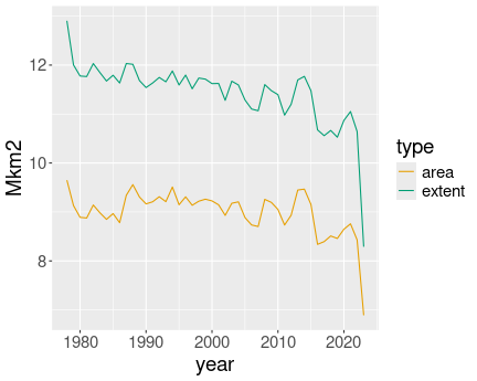
Yearly average ice extent and area over time.
ice %>%
group_by(year) %>%
summarize(extent = mean(extent),
area = mean(area)) %>%
pivot_longer(c(extent, area),
values_to = "Mkm2",
names_to = "type") %>%
ggplot(aes(year, Mkm2,
col = type)) +
geom_line()Note that we might get the same results differently, by using
geom_line() twice, first with with aesthetics mapping
aes(year, extent) and thereafter
aes(year, area). Note also that the first and last averages
may be off, depending on which months are included/excluded for those
years.
K.15 Making maps
K.15.1 Shapefiles and GeoJSON
K.15.1.1 Difference between spatial data frame and manual map data frame
There are multiple differences:
- Perhaps most importantly, the hand-made NZ map in Section 16.1.1 is stored as one vertex per row, while the spatial data frame is stored one polygon per row. This makes spatial data frames much smaller, for instance, you do not need to replicate the same color value for every single vertex–a single value for the polygon is enough.
- Another important difference is the presence of coordinate reference system (CRS). This allows to easily transform one coordinate system to another, and in this way to use spatial data that is stored using different systems.
K.15.1.2 Why all.x = TRUE?
This is because we want to retain all rows of map but drop the lines of population where there are no corresponding region on the map. Hence we retain all regions (rows of map), with potentially NA as the population value. This is a reasonable approach.
Alternatively:all = FALSE) (inner join) would remove regions where population from the map. That would leave holes in the map for those places where we do not have population data. It is probably better to keep those regions and use a dedicate NA-color, such as gray, instead.all = TRUE(outer join) will preserve all regions, but also population information for those regions that are not present on the map. This will probably not be a serious problem, it may just clutter your data frame with un-necessary rows.- finally,
all.y = TRUE(right join) will combine the worst of both worlds: leave holes in map for missing population data, while also cluttering the final dataset.
K.16 Machine Learning
K.16.1 \(k\)-nearest neighbors
K.16.1.1 Iris decision boundary plot
- First, create the predictor matrix (design matrix) X and the label vector label:
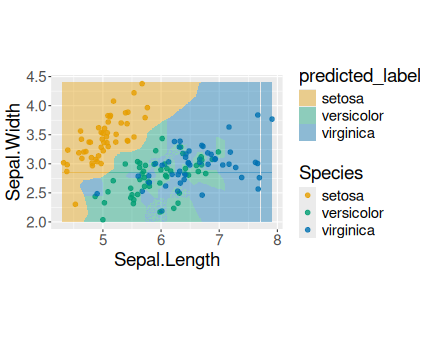
library(class)
nGrid <- 200
## 200 points between smallest
## and largest valuee
ex <- data.frame(
Sepal.Length = seq(min(X$Sepal.Length),
max(X$Sepal.Length),
length.out=nGrid))
ey <- data.frame(
Sepal.Width = seq(min(X$Sepal.Width),
max(X$Sepal.Width),
length.out=nGrid))
grid <- merge(ex, ey)
predicted_label <- knn(X, grid, cl = label,
k = 1)
iris %>%
ggplot(aes(Sepal.Length, Sepal.Width,
col = Species)) +
geom_jitter(size = 2, alpha = 0.8) +
coord_fixed() +
geom_tile(data = grid,
aes(fill = predicted_label),
col = NA, # no border
alpha = 0.4)In this plot I have used geom_jitter() instead of geom_point() to
avoid overplotting the same datapoints.
You can remove the double legend by e.g. adding + guides(fill = "none").
Based on this plot, virginica and versicolor are hard to
distinguish. But setosa is clearly different from both of these.
- When using sepal length and petal width, it is easier (but not trivial) to distinguish between virginica and versicolor. Setosa is again very different.
K.17 Data structures
K.17.1 Factor Variables
K.17.1.1 Age as unordered/ordered factor
First, let’s compute the averages across trees:
orange <- read_delim("data/orange-trees.csv")
avgs <- orange %>%
group_by(age) %>%
summarize(size = mean(circumference))
avgs## # A tibble: 7 × 2
## age size
## <dbl> <dbl>
## 1 118 31
## 2 484 57.8
## 3 664 93.2
## 4 1004 134.
## 5 1231 146.
## 6 1372 173.
## 7 1582 176.As you see, by default the grouping variable age is numeric (dbl). Hence by default, ggplot would paing the bars in different shades of blue. Also, the numeric values will be naturally ordered by default, so you do not need to specify the levels and their order when converting it to an ordered factor.
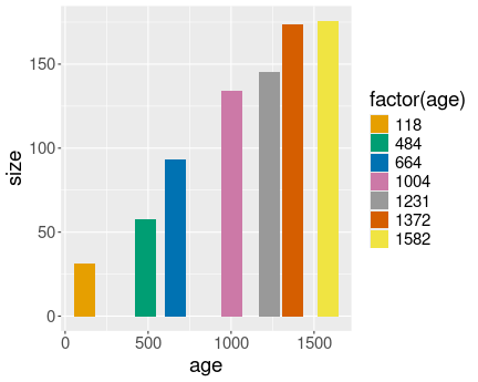
Orange tree growth. age as unordered factor, and hence filled with unrelated contrast colors.
Here we convert age to (unordered) factor. Here ggplot uses contrast colors that are not ordered in any way:
Although the picture does the job, the colors look incoherent.
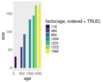
Orange tree growth, but now age values are ordered. ggplot picks an gradient color scale.
When forcing age to be ordered, we get a much more pleasant and meaningful result:
Here a gradient scale, the default for ordered factors, makes much more sense, but you may want to change the legend key title (or remove the key completely).