Chapter 6 Vectors
This chapter covers the foundational concepts for working with vectors in R. Vectors are the fundamental data type in R: in order to use R, you need to become comfortable with vectors. This chapter will discuss how R stores information in vectors, the way in which operations are executed in vectorized form, and how to extract subsets of vectors. These concepts are key to effectively programming in R.
While keeping all data in vectors is specific to R, many programming languages support similar vectors in one form or another. Vectors and vectorized operations are also fundamental tools for data programming.
6.1 What is a Vector?
Vectors are simply a number of similar values stored next to each
other. For example, you can make a vector that contains the
character strings “Sarah”, “Amit”, and “Zhang”. As another example, you
can make a vector that stores the numbers from 1 to 100. In R,
vectors are just ordinary variables, so you can call the vector of
three persons people and the vector of 100 integers numbers.
Technically, vectors are one-dimensional ordered collections of
values that are all stored in a single variable. Each value in a
vector is refered to as an element of that vector; thus the
people vector would have 3 elements, "Sarah", "Amit", and
"Zhang", and numbers vector will have 100 elements. Ordered
means that once in the vector, the elements will remain there in the
original order. If “Amit” was put on the second place, it will remain
on the second place unless explicitly moved.
Unfortunately, there are at least five different and sometimes contradicting definitions of what is “vector” in R. Here we focus on atomic vectors, vectors that contain the atomic data types (see Section 4.4). Another different class of vectors is generalized vectors or lists, the topic of Section 8.
Atomic vector can only contain elements of a single atomic data type—numeric, integer, character or logical. Importantly, all the elements in a vector need to have the same. You can’t have an atomic vector whose elements include both numbers and character strings.
6.2 Creating Vectors
6.2.1 Combining elements with c()
Perhaps the most straightforward and universal way to create
vectors is to use the built in c() function, which c_ombines_
values into a vector. The c() function takes in any number of
arguments of the same type (separated by commas as usual), and returns a vector that contains those elements:
## [1] "Sarah" "Amit" "Zhang"## [1] 1 2 3 4 5You can use the length() function to determine how many elements are in a vector:
## [1] 3## [1] 5As atomic vectors can only contain same type of elements, c()
automatically casts (converts) one type to the other if necessary
(and if possible). For instance, when attempting to create a vector
containing number 1 and character “a”
## [1] "1" "a"we get a character vector where the number 1 was converted to a character “1”. This is a frequent problem when reading data where some fields contain invalid number codes.
c() can also be used to add elements to an existing vector:
# Use the combine (`c()`) function to create a vector.
people <- c("Sarah", "Amit", "Zhang")

# Use the `c()` function to combine the `people` vector and the name 'Josh'.
more_people <- c(people, 'Josh')
print(more_people)  # [1] "Sarah" "Amit"  "Zhang" "Josh"
Note that c() retains the order of elements—“Josh” will be the
last element in the extended vector.
c() can also combine several vectors:
## [1] 1 2 3 3 2 1 1 2 3produces a sequence of three sequences. In fact the previous example
did the same–remember that "Josh" is just a character vector
of length 1.
6.2.2 Creating sequences
We frequently need to create vectors that contain numbers in regular
intervals. Section 5.1 used one of such tools, namely
creating integer sequences with the colon operator : like
## [1] 1 2 3 4 5 6 7 8 9 10Now it is time to talk about the leading [1] in the printout. This
means that the printout here starts with the first component of the
vector. If the whole vector does not fit into a single line, it will
be split into multiple lines, and each line starts with a similar
bracketed number, telling which element
(which index,
see Section 6.4 below)
is the first one in the
corresponding row. For instance, if printout is narrow, you may see
##  [1]  1  2  3  4  5  6  7  8
##  [9]  9 10 11 12 13 14 15 16
## [17] 17 18 19 20
Here the first row starts with the 1st element, second row with 9th element, and the third row with the 17th element. This makes the output more readable, so you know where in the vector you are when looking at a line of output!
The colon operator is actually a shortcut for seq()
function. seq() takes at least two arguments, from and to, and
creates and integer sequence between these values. For instance
## [1] 1 2 3 4 5 6 7 8 9 10## [1] 10 9 8 7 6 5 4 3 2 1But seq() allows additional functionality, e.g. the step (by), or
the total length (length.out =)
## [1] 1 3 5 7 9## [1] 0.0 0.5 1.0 1.5 2.0 2.5 3.0 3.5 4.0 4.5Exercise 6.1 You have a dataset of monthly observations. It starts with February 1985, and it includes 350 rows in total, and each row corresponds to a month.
Write a sequence that shows which row corresponds to April observations. Ensure that you do not go past the total number of rows!
Hint: the first April is in row 3.
See the solution
6.2.3 Replicating elements with rep()
Another useful function that creates vectors is rep() that repeats
it’s first argument:
All functions for creating vectors we introduced here, c(), seq() and
rep(), are noticeably more powerful and complex than the brief
discussion above. Check out the documentation!
6.3 Vectorized Operations
Many R operators and functions are optimized for vectors, i.e. when fed a vector, they work on all elements of that vector. These operations are usually very fast and efficient.
6.3.1 Vectorized Operators
A lot of common operators, such as +, -, are vectorized–when
applied to a vector, they work on all elements of the vector. More
precisely, these operations are performed by the elements that are in
the same position in the first and in the second vector.
For instance, if you want to add (+) two vectors, then the value of
the first element in the result will be the sum (+) of the first
elements in both “addend” vector, the second element in the result
will be the sum of the second elements in both “addend”, and so on.
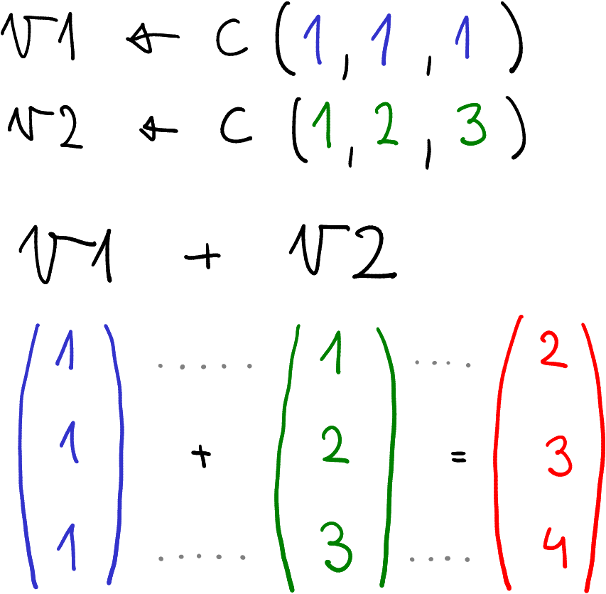
Adding two vectors, element-wise
For instance, if we take two vectors (see the figure),
their sum is
## [1] 2 3 4This is because all elements at the corresponding positions are added, to get the final vector.
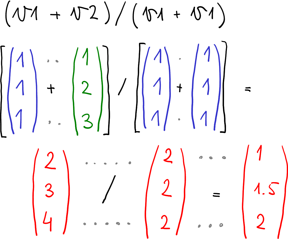
More complex vectorized operations are also performed element-wise.
More complex vectorized operations are computed element-wise in a
similar fashion. For instance, let’s compute (v1 + v2)/(v1 + v1).
First we need to compute v1 + v2 and thereafter v1 + v2, both of
these element-wise. Finally, we perform the division, again
element-wise:
## [1] 1.0 1.5 2.0Such vectorized operations are usually fairly intuitive and do not cause many problems. Logical operations, however, are a bit less intuitive, although they work in exactly the same manner.
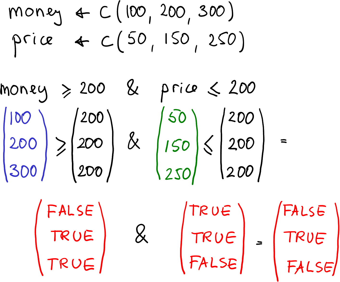
Logical operations are vectorized in exactly the same manner.
Imagine you decide whether to get a puppy. You’ll only get it if you have at least $200 money, and if puppy costs no more than $200. In the first day, you only have $100 while the puppy is cheap, just $50. The next day you have $200 and the puppy costs $150; and the third day you have $300 but now the puppy costs $250. You can put these values into vectors as
The logical operation, whether to buy the puppy, can be written as
## [1] FALSE TRUE FALSEThe individual operations are done element-wise, exactly as with arithmetic operators. Here, essentially, all these operations are done separately for each different day.
Finally, note that similar vectorized operations also exist in many other programming languages.
Exercise 6.2 Three customers are coming to a liquor store, aged 16, 20 and 24, and want to buy a drink. The first and the third customer are served by cashier called Yu Huang, the second one by one, called Guanyin. Yu Huang will not sell any liquor to those under 21, but Guanyin is willing to sell to anyone.
- Put the customer ages and cashier names in appropriately named vectors
- Explain the condition in words: who will be able to buy the drink? And which customers are those?
- Write a logical expression about the above. This should result in True for those able to buy the drink and False for those who are not able to buy.
See the solution
6.3.2 Vectorized Functions
Vectors In, Vector Out
Because all atomic objects are vectors, it means that pretty much every
function you’ve used so far has actually applied to vectors, not just to
single values. These are referred to as vectorized functions, and
will run significantly faster than non-vector approaches. You’ll find
that functions work the same way for vectors as they do for single
values, because single values are just instances of vectors! For
instance, we can use paste() to
concatenate the elements of two character vectors:
colors <- c("Green", "Blue")
spaces <- c("sky", "grass")

# Note: look up the `paste()` function if it's not familiar!
paste(colors, spaces)  # "Green sky", "Blue grass"
Notice the same member-wise combination is occurring: the paste() function is applied to the first elements, then to the second elements, and so on.
Fun fact: The mathematical operators (e.g.,
+) are actually functions in R that take 2 arguments (the operands). The mathematical notation we’re used to using is just a shortcut.
For another example consider the round() function described in the previous chapter. This function rounds the given argument to the nearest whole number (or number of decimal places if specified).
But recall that the 1.6 in the above example is actually a vector of
length 1. If we instead pass a longer vector as an argument, the function will perform the same rounding on each element in the vector.
# Create a vector of numbers
nums <- c(3.98, 8, 10.8, 3.27, 5.21)

# Perform the vectorized operation
round(nums, 1)  # [1]  4.0  8.0 10.8  3.3  5.2
This vectorization process is extremely powerful, and is a significant factor in what makes R an efficient language for working with large data sets (particularly in comparison to languages that require explicit iteration through elements in a collection). Thus to write really effective R code, you’ll need to be comfortable applying functions to vectors of data, and getting vectors of data back as results.
Remember: when you use a vectorized function on a vector, you’re using that function on each item in the vector! Vectorized operations work element-wise.
6.3.3 Summary functions
Previously we looked at a number of vectorized functions that operated
elementwise–“vector-in, vector out”. But there is also a large class
functions that are vectorized in a different way–“vector in, a single
number out”. This includes functions such as sum() (add all
elements of a vector), min() (find the minimum element), or
str_flatten() in the stringr library (combine all elements of a
string vector together).
Here a few examples:
## [1] 55## [1] 1## [1] 5.5All these functions transformed a vector into a single number.
String concatenation belongs to the same category:
library(stringr)
words <- c("once", "upon", "a", "time")
str_flatten(words, collapse=" ")  # put " " between words
## [1] "once upon a time"Another similar function is range() that returns the minimum and
maximum:
## [1] 1 10Although it returns a vector–both minimum and maximum, it still belongs to the summary function category. This is because it always returns just two elements, no matter how long is the input vector. Just it summarizes the vector in two numbers, not in a single one.
These functions are often used to compute a single summary statistic of data.Exercise 6.3 Summary statistics. Consider vectors
For each of these vectors, compute a) mean; b) median (function
median()); c) range; and
d) variance (function var()).
How similar/different are these figures?
See the solution
6.3.4 Recycling
Above we saw a number of vectorized operations, where similar operations were applied to elements of two vectors member-wise. However, what happens if the two vectors are of unequal length?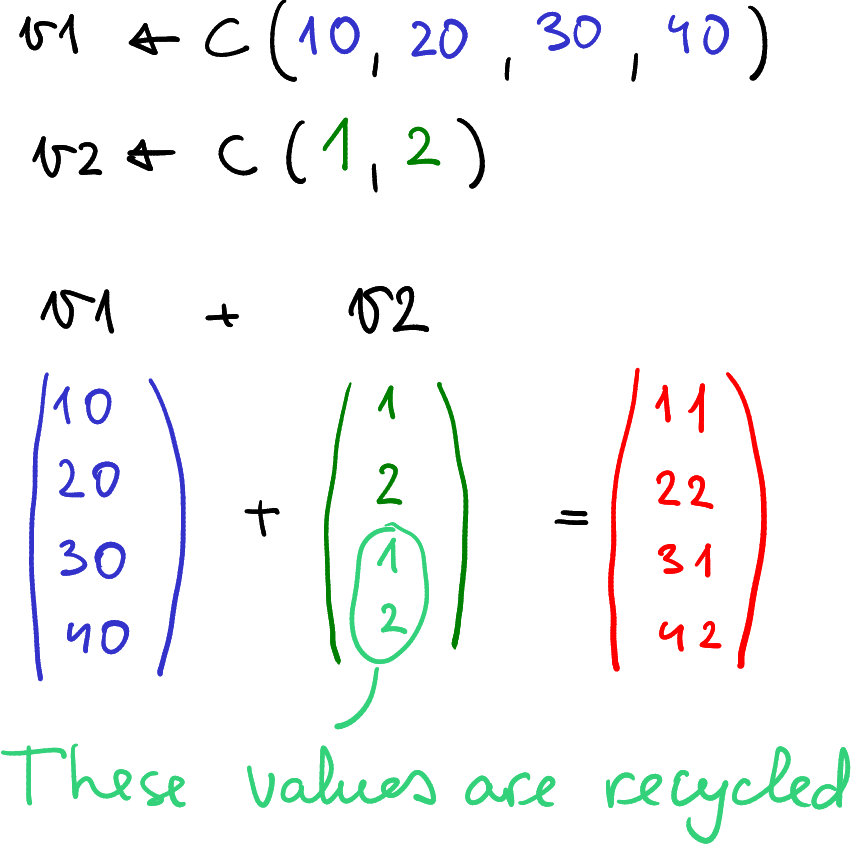
Recycling: the shorter vector v2 of length 2 is “recycled” one more
time to match the longer vector of length 4.
In that case R uses recycling rules: the shorter vector is repeated, potentially many times, to match the longer one. For example:
## [1] 11 22 31 42In this example, R first combines the elements in the first position of
each vector (10 + 1 = 11). Then, it combines the second
position (20 + 2 = 22).
When it gets to the third element of v1 it run out
of elements of v2, so it went back to the beginning of v2 to
select a value, yielding 30 + 1 = 31. Finally, it add the 4th element
of v1 (40) to the second element of v2 (2) to get 42.
If the longer object length is not a multiple of shorter object length, R will issue a warning, notifying you that the lengths do not match. This is a warning, not an error, but in practice it almost always means you have done something wrong.
Exercise 6.4 What is the exact warning message? What is the result?
Try adding c(10, 20, 30, 40) and c(1, 2, 3).
See the answer
Actually, we have already met many examples of recycling and vectorized functions above. For instance, in Section 6.3.1 we computed
In fact, here we actually recycle “200” for three times, so the actual
operation looks like c(100, 200, 300) >= c(200, 200, 200).
The result is a logical
vector of length 3.
This is also what happens if you add a vector and a “regular” single value (a scalar):
## [1] 2 3 4As you can see (and probably expected), the operation adds 1 to every
element in the vector. The reason this sensible behavior occurs is
because all atomic objects are vectors. Even when you thought you were
creating a single value (a scalar), you were actually just creating a
vector with a single element (length 1). When you create a variable
storing the number 7 (with x <- 7), R creates a vector of length 1
with the number 7 as that single element:
This is why R prints the
[1]in front of all results: it’s telling you that it’s showing a vector (which happens to have 1 element) starting at element number 1.This is also why you can’t use the
length()function to get the length of a character string; it just returns the length of the array containing that string (1). Instead, use thenchar()function to get the number of characters in each element in a character vector.
Thus when you add a “scalar” such as 4 to a vector, what you’re really doing is adding a vector with a single element 4. As such the same recycling principle applies, and that single element is “recycled” and applied to each element of the first operand.
Note: here we are implicitly using the word vector in two different meanings. The one is a way R stores objects (atomic vector), the other is vector in the mathematical sense, as the opposite to scalar. Similar confusion also occurs with matrices. Matrices as mathematical objects are distinct from vectors (and scalars). In R they are stored as vectors, and treated as matrices in dedicated matrix operations only.
Finally, you should also know that there are many kinds of objects in R that are not vectors. These include functions, formulas, environments, and other “exotic” objects.
6.4 Vector Indices
Vectors are the most important data structure for storing data in R. Yet often you want to work only with some of the data in the vector, not with the complete vector. This section will discuss the main ways how you can extract and modify a subset of elements in a vector.
6.4.1 Numeric Index
Perhaps the most intuitive way to access individual elements is to refer to them by just their position. For example, look at the vector:
## [1] "a" "e" "i" "o" "u"Here element 'a' is at the position 1, 'e' is at position 2, and so on.
You can retrieve the elements by using bracket notation: you refer
to the element at a particular position by writing the name of the
vector, followed by square brackets ([]) that contains the
position(s) of interest:
## [1] "a"## [1] "i"Don’t get confused by the [1] in the printed output—it doesn’t
refer to the position where you got the vowel from, but the position
in the extracted result.
R vector elements are indexed starting with “1” (called one-based indexing). This is distinct from many other programming languages which use zero-based indexing where the first position is “0”. Both approaches have their advantages.
If you specify a position that is out-of-bounds (e.g., greater than
the number of elements in the vector) in the square brackets, you will
get back the value NA, which stands for Not Available.
## [1] NANote
that this is not the character string "NA", but a specific value,
specially designed to denote missing data. See more in Section
12.6.
If you specify a negative position in the square-brackets, R will return all elements except the (negative) one specified:
## [1] "a" "i" "o" "u"It is important to be aware that what we do here does not modify the vector itself: the vector vowels is unchanged after all these operations:
## [1] "a" "e" "i" "o" "u"The operations created a new vector that was printed, but not stored.
If we want to eliminate an element from vowels, we need to a)
eliminate it with negative index; and b) store it back to vowels
using <-:
## [1] "a" "e" "o" "u"See more in Section 6.5.
6.4.2 Multiple Indices
Above, we extracted (or removed) single elements only. But we can use numeric vectors to extract or eliminate multiple elements in one go. Let’s do the examples with character vectors this time:
First, we may specify the positions of the colors as a separate index vector:
## index vector
i <- c(2, 1, 4)
## Retrieve the colors at those positions
colors[i]  # note: 'gold' first, 'purple' second
## [1] "gold" "purple" "black"This is a good approach if the index vector is complicated, possibly calculated somehow.
Other times we may just specify the positions directly without any dedicated index vector:
## [1] "gold" "gray"This is a good way to work with simple index vectors like the one above.
The colon operator to specify a sequences is a popular helper tool for element extraction (see Section 6.2):
## [1] "gold" "white" "black" "gray"This easily reads as “a vector of the elements in positions 2 through 5”.
The object returned by indexing is a copy of the original, unlike in some other programming languages. These are good news in terms of avoiding unexpected effects: modifying the returned copy does not affect the original. However, copying large objects may be slow and sluggish.
There are other ways to extract elements, e.g. functions head() and
tail() extract a given number of elements from the beginning or from
the end of the vector. Look up the corresponding documentation.
6.4.3 Logical Indexing
Numeric indexing we did above is good if you know the exact position of the elements of interest. But very often, it depends on the actual values. This is where logical indexing comes in super handy.
Imagine that you are the administrator of an affordable housing project. The rules stipulate that the apartments are only available to applicants whose income is less than 60 ($1000 per year). You have five applicants with incomes
## [1] 30 45 70 110 55Now we will write code to decide which applicants will be able to rent a
place.
The numeric index we use above work, e.g. incomes[c(1,2,5)] will
give the list of eligible applicants. But as soon as your staff
shuffles around the applications, or a new application is coming in,
the index vector c(1,2,5) is not valid any more.
The solution to the consistency problem is to use logical values as index, and let the computer to calculate these values. This is logical indexing. First, we do it manually (this feels clunky), and thereafter we let computer to calculate the correct index (this is extremely useful).
Logical index is just a logical vector of the same length as the
income vector where TRUE in the to extract and
FALSE means not to extract the element at the corresponding
position.
Out of the
applicants, the 1st, 2nd and 5th have income below the threshold, so
we can write
index <- c(TRUE, TRUE, FALSE, FALSE, TRUE)
                           # extract 1st, 2nd, 5th, leave out 3rd, 4th
incomes[index]
## [1] 30 45 55R will go through the logical index vector and extract every item at the
position that is TRUE. In the example above, since index is TRUE
at positions 1, 2, and 5,
incomes[index] returns a vector with the elements from positions
1, 2, and 5. This is the basics how logical indexing works, but when
used manually like what we did here, it is not a very useful tool.
But this tool becomes incredibly powerful when we let R to compute the logical index vector. This allows us to specify certain criteria that the vector elements (data) must satisfy, and select only those elements. This process is called filtering, and we will do a lot of filtering later with data frames. In order filter, you first need to create the logical index vector by logical conditions your data must satisfy, and thereafter you it for logical indexing. So instead of manually specifying whether each applicant fall within the required income bracket, we let R to compute it. We can write:
## [1] TRUE TRUE FALSE FALSE TRUE## [1] 30 45 55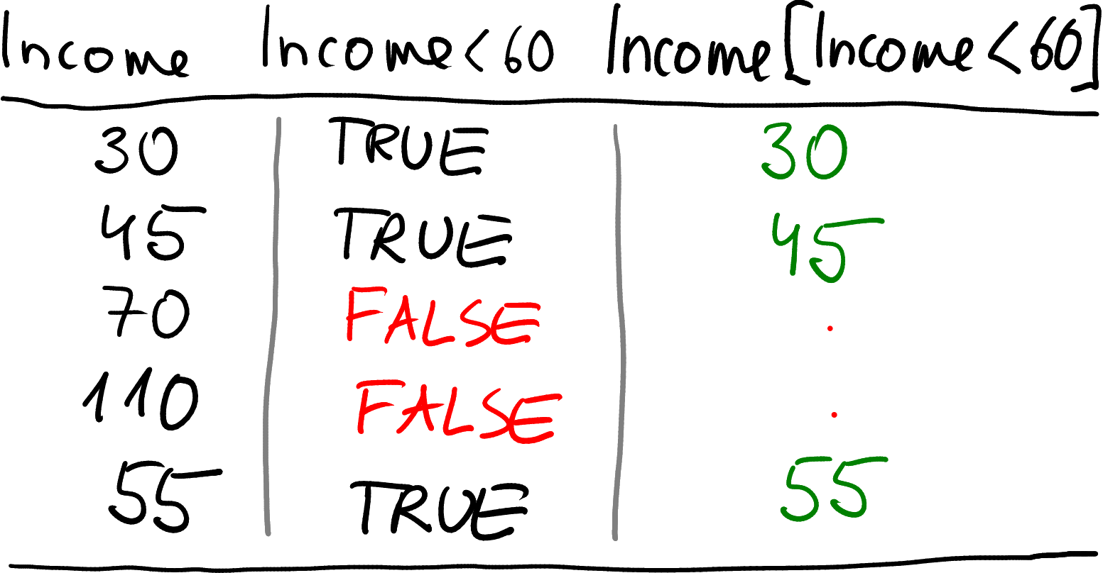
How logical indexing works. The condition Income < 60 will be
evaluated to TRUE, TRUE, FALSE, FALSE, TRUE, corresponding
to the income values. Thereafter, only those values that correspond
to TRUE are retained (green) while those corresponding to FALSE are
dropped (red dots). At the end we have a vector of three elements:
30, 45 and 55.
There is often little reason to explicitly create the index vector
index. We can just write the filtering criterion directly inside
square brackets:
## [1] 30 45 55Figure at right explains how the computation works. First, R computes
the logical vector incomes < 60 and gets a series of TRUE-s and
FALSE-s. Thereafter, this logical vector is used to extract certain
elements from incomes, the elements corresponding to FALSE are
dropped.
You can think of this statement as “tell me income where income is less than 60”.
Why is this approach better than numeric indexing? Because now the
code does not change when the number of applications and their order
changes. Your staff may shuffle around the applications as they
wish, and many more may come in at the last moment, but the code,
incomes[incomes < 60], will still do its job as expected.
This kind of filtering is immensely popular in real-life applications.
Exercise 6.5 Create a vector -5, -4, -3, … 3, 4, 5. Extract only positive numbers from it.
See the solution
Note that the index can be computed based on a different vector than the one where we are extracting the elements from. For instance, instead of incomes, we may want to extract the eligible applicants’ names. Now we need two vectors of data:
incomes <- c(30, 45, 70, 110, 55)  # $1000 per year
names <- c("Xuanzhang", "Sha Wujing", "Yu Huang", "Guanyi", "Buddha")
The names of the eligible applicants can be extracted as
## [1] "Xuanzhang" "Sha Wujing" "Buddha"This can be understood as follows: first, incomes < 60 creates
a logical vector
for eligible applicants. This is exactly the same procedure we did
above. Next, we use the logical vector as logical index, but now we
extract elements from names, not from incomes. The idea is very
similar though.
Exercise 6.6 You are working in a hospital with patents’ data:
height <- c(160, 170, 180, 190, 175)  # cm
weight <- c(50, 60, 70, 80, 90)  # kg
name <- c("Kannika", "Nan", "Nin", "Kasem", "Panya")
Extract: * height of all patients who are at least 180cm tall * names of all patients who are at least 180cm tall * weight of all patients who are at least 180cm tall * names of everyone who weighs less than 70kg * names of everyone who is either taller than 170, or weighs more than 70.
See the solution
6.4.4 Named Vectors and Character Indexing
All the vectors we created above where made without names. But sometimes it is handy to give each element a name. For instance, we may have a vector of student grades and we can use the names to tell whose grade is it. We can create such a vector as
##      Dai      Bao Tan-chun Bao-chai
##      4.0      3.9      3.8      3.7
This creates a numeric vector of length 4 where the elements have
values 4.0, 3.9, 3.8 and 3.7. However, this is not all that the
vector has, now the elements also have names.
Note that the printout differs from that
of unnamed vectors, in particular the index position ([1]) is not
printed. Such way of creating a named vector is good when we
have a few values only.
If the vector component has a name that is a valid R variable name
(see Section 4.3.2), then you can just assign it as
c(Dai = 4), just as if using a named argument. However, if the name
is not a valid variable name, then you need to quote it either with
backtics like
c(`Tan-chun` = 3.8) or with quotes, as for Bao-chai.
This is because Tan-chun
and Bao-chai contain a dash and
cannot normally be used as a variable name. As the same approach–quoting
invalidvariable names with backtics–also applies to data frames,
we’ll use that approach here.
Using such a named vector makes it very easy to access elements based on the name. For instance, Dai’s and Tan-chuns grades can be read as
##      Dai Tan-chun
##      4.0      3.8
We use a character vector for indexing. We can create it explicitly as above, or create it on-the-go without naming it as
##      Dai Tan-chun
##      4.0      3.8
Alternatively, we can set names to an already existing vector using the
names()
function:21
This is a good approach when we have a large number of values, too tedious to be named manually.
Now when we have a named vector, we can access it’s elements by names. For instance
Note that in the latter case the names "B" and "D" are in “wrong
order”, i.e. not in the same order as they are in the vector numbers.
However, this works just fine, the elements are extracted in the order
they are specified in the index (This is only possible with character
and numeric indices, logical index can only extract elements in the
“right” order.)
While most vectors we encounter in this book gain little from names, exactly the same approach also applies to lists and data frames where character indexing is one of the important workhorses.
Another important use case of named vectors in R are a substitute of maps
(aka dictionaries). Maps are just lookup tables where we can
find a value that corresponds to a value of another element in the
table. For instance, the example above found values that correspond to
the names "D" and "B".
Exercise 6.7 Use data about the US states (see Section I.20): the
built-in variable state.abb contains the state name abbreviation
(such as “WA” for “Washington”) and state.name contains the full
name.
- create a named vector of the state name abbreviations that has full state names as its names.
- Use character indexing to extract abbreviations for Utah, Connecticut, and Nevada. Do this in a single line of code!
See the solution
6.5 Modifying Vectors
Indexing is the prime tool when we want to modify elements within the vector.22 Modification is easier if all desired elements will be replaced by the same value, and slightly more elaborate if every element needs to have a different value.
6.5.1 Basics of modifying vectors
In order to replace a subset of elements in a vector, place the extracted subset on the left-hand side of the assignment operator, and then assign them a new value. Here we replace “pen” with “pencil” in a supplies vector:
supplies <- c("backpack", "laptop", "pen")
supplies[3] <- "pencil"  # replace the third element (pen)
                           # with 'pencil'
supplies
## [1] "backpack" "laptop" "pencil"And of course, there’s no reason that you can’t select multiple elements on the left-hand side, and assign them multiple values. The assignment operator is vectorized! But if you want to replace, for instance, two elements, you need to also supply two elements
## Replace  'laptop' with 'tablet', and 'pencil' with 'book'
supplies[c(2, 3)] <- c("tablet", "book")
supplies
## [1] "backpack" "tablet" "book"Exercise 6.8 What happens if you give the vector a different number of items to replace? Try using a single item
and 3 items
See the solution
If the vector has names, you can use character indexing in exactly the same way as the numeric index.
6.5.2 The same value for all replaced elements
Logical indexing offer some very powerful possibilities. Imagine you had a vector of values in which you wanted to replace all numbers greater that 10 with the number 10 (to “cap” the values). We can achieve with an one-liner:
v1 <- c(1, 5, 55, 1, 3, 11, 4, 27)
tooLarge <- v1 > 10  # logical index: which element is > 10?
tooLarge
## [1] FALSE FALSE TRUE FALSE FALSE TRUE FALSE TRUE## [1] 1 5 10 1 3 10 4 10In this example, we first compute the logical index of “too large”
values by v1 > 10, and thereafter assign the value 10 to all these
elements in vector v1.
Obviously, we do not need to create a separate index vector, we can
just do instead
This will result in exactly the same outcome, and it is a very widely used construct in R.
6.5.3 Different value for different elements
The above example replaced all too large values with the same number, “10”. But what if we want to replace different values with different numbers? Let’s look at four managers, Shang, Zhou, Qin and Han. We create a named vector (see Section 6.4.4) of their income. Names are not needed here, but they help to make the calculations more explicit:
## Shang  Zhou   Qin   Han
##  1000  2000  3000  4000
Up to now, they had to pay a proportional tax rate of 10% of their income:
## Shang  Zhou   Qin   Han
##   100   200   300   400
However, now the government introduces a progressive tax: wealthy people, those with income over 2500, have to pay 20%, the “top tax rate”. How can we modify the tax vector accordingly? We can do it explicitly in multiple steps: first find who is wealthy, then compute the top tax amount, and then replace the tax for the wealthy by the high tax amount for the same persons:
iWealthy <- income > 2500  # who is wealthy?
topTax <- 0.2*income  # the top tax (only applies for wealthy)
tax[iWealthy] <- topTax[iWealthy]  # replace the tax for the wealthy only
tax
## Shang Zhou Qin Han
## 100 200 600 800Now the poor Shang and Shou still pay what they paid before, but the wealthy Qin and Han pay the double than what they paid earlier.
Note how we use the logical index, iWealthy on both sides of the
assignment: at left, it tells that we only want to overwrite the tax
of the wealthy, and at right, it tells that only use the new tax
amounts for the wealthy for overwriting.
Obviously, this can be done in a more concise manner, e.g.
This is a very frequently used construct in R.
Exercise 6.9 Implement absolute value: consider a vector of both positive and negative numbers, and 0:
Replace negative elements in this vector with the corresponding positive ones, so it will be
Use the element replacement tools you learned in this section.
See the solution
Exercise 6.10 Consider the four managers above again. Their income is as before:
Now they also have to pay rent. They pay
The government introduces housing benefits for the rent-burdened: everyone who is paying more than 50% of their income for rent, will get a benefit \[\begin{equation} b = \frac{1}{4} \mathit{rent}. \end{equation}\] Those who pay less rent, will receive nothing. How much of a benefit will each of them get?
Compute the vector of benefits in the following manner:- Assign benefit “0” to everyone;
- Replace the benefit of those who are rent-burdened with the benefit computed by the formula above.
See the solution
6.6 Computing with vectors
There are a number of compute tasks we often want to do with vectors. This includes summing and multiplying its elements, finding number of elements that match certain criterion, or the percentage of such elements. Here we discuss counting elements that match criteria, summing was explained above in Section 6.3.3.
Let’s be simple and analyze odd numbers among numbers 1..11:
Remember, “oddness” can be tested as the modulo when dividing by 2 is 1:
## [1] TRUE FALSE TRUE FALSE TRUE FALSE TRUE FALSE TRUE FALSE TRUEThis results in a logical vector where True corresponds to odd numbers. The two tasks below involve this logical vector.
How many elements match a criterion. This is just the count of True’s in the logical vector. A straightforward but not-so-smart way is to select just the odd elements, and find the length of the final vector:
## [1] 6This gives the correct number, 6. But why is it not so smart?
This is because there is a simpler way of getting the same result:
## [1] 6How does sum() achieve the same result? This is because logical
values are automatically converted to numbers as soon as you do some
math with these. And they are converted in a way that TRUE will be
“1” and FALSE will be “0” (see also Section
4.4.3).
So, summing a logical vector means
summing Trues as zeros won’t count anyway.
But summing ones is as good as
counting. This is how sum of a logical vector equals the count of
Trues.
What percentage of elements match the criterion is somewhat analogous. As percentage is just sum divided by number of cases, one may want to divide the number of cases that match with the number of all cases:
## [1] 0.5454545The answer is correct but again, the method is not smart. It is better to use
## [1] 0.5454545How does this work? In very much the same way. The function mean()
is a dedicated function to compute averages, i.e. compute sum and
divide by the number of elements. Hence it computes the sum exactly
the same way as we did above, but now it also does the division for
you.
These small tricks are both easier to code, easier to read, and also
less error-prone. The same tricks also works in other programming
languages besides R, the only requirement is that it has functions
like sum() and mean() that operate on vectors, and logical values
are translated to numbers in a similar fashion.
Use these when writing code!
6.7 Looping over vector elements
Through the course we try hard to make you to use vectorized operations instead of loops as those are more efficient, easier to write and less error-prone. But there are many tasks that cannot be easily vectorized, and in those cases a loop over vector elements may be the best option.
6.7.1 Accumulate values into a vector
Sometimes we want to run a loop over a sequence, be these just numbers or something more complex, like data files. Each time we compute a value and add it to the vector. Here a simple example that creates a vector of squares of integers:
s <- c()  # start with an empty vector (accumulator)
for(n in 1:10) {
   s <- c(s, n^2)  # add n^2 to the end of the vector
}
s  # all squares
## [1] 1 4 9 16 25 36 49 64 81 100Such loop is just a special case of accumulating values (see Section
5.1.2). c() is the “empty basket”; picking the
berry here means computing the next square; and putting it in basket
is done using c(s, n^2).
Such approach is not well suited for this particular task–(1:10)^2
will be shorter, faster, and easier to read. But the method is more
general and applies to situations that are hard to vectorize. For
instance, you may have to loop over different datasets, each time loading
the file and perform some data processing to come
up with a value of interest. In such cases a loop is a much cleaner
approach than brute-force vectorization.
Instead of loops, you
can also use the lapply() family of functions (see Section
20.5).
Here is an example, using function integrate() that is not
vectorized. For instance,
\[\begin{equation}
\int_0^a \mathrm{e}^{-x} \, \mathrm{d} x
\end{equation}\]
where \(a = 1\) can be calculated as
a <- 1
## Define the function
f <- function(x) {
   exp(-x)
}
integrate(f, 0, a)  # arguments are: function, lower bound, upper bound
## 0.6321206 with absolute error < 7e-15It returns a list, where the component $value gives the numeric
value, here 0.6321206 (see Section 8 for more about
lists). Just by default, the list is printed in a nice way, so you
cannot see what exactly does integrate() return.
integrate() requires \(a\) to be a single number, not a vector:
## Error in integrate(f, 0, as): length(upper) == 1 is not TRUEThis is a place where where we may want to use a for-loop instead:
as <- 1:5
Is <- c()  # start with an empty vector
for(a in as) {
   Is <- c(Is,
           integrate(f, 0, a)$value)  # exctract the numeric 'value'
               # Add it to the Is vector
}
Is  # 5 numbers, corresponding to the 5 upper bounds
## [1] 0.6321206 0.8646647 0.9502129 0.9816844 0.9932621Another reason to prefer accumulating elements to a list is the case where you do not want to accumulate all of them. For instance, let’s compute square roots of numbers, and only preserve integers where \((\sqrt{n})^2 \not = n\), \(n \in \mathbb{Z}^+\). While the equation is always true in the mathematical sense, computers cannot compute square roots and products precisely, and hence we expect this not to be TRUE in general. For instance:
## [1] 4.440892e-16Here is a loop that runs over numbers 1 to 25, and preserves only those where the identity is not TRUE:
wrongZ <- c()
for(z in 1:25) {
   if(sqrt(z)^2 != z) {
               # only include z to the list if the calculation
               # gives an incorrect result
      wrongZ <- c(wrongZ, z)
   }
}
wrongZ
## [1] 2 3 5 6 7 8 10 12 13 15 18 19 20 23 24As you see, the list includes most numbers which’ square root is not an integer, but peculiarly, 11, 14, 17, 21 and 22 are missing. Apparently in those cases the errors cancel out.
Note that here you could also use a vectorized operation:
(1:25)[sqrt(1:25)^2 != 1:25] instead. But in other cases this may
not be so. For instance, if you want to test if a number is prime,
you cannot write this down easily as vectorized operations.
Alternatively, if you are testing a very long list of values, it may
be more efficient to store in memory
only the few numbers we need, not the whole array.
Exercise 6.11 Create a list of odd numbers between 1 and 10 in the following way:
- loop over all integers between 1 and 10
- test if the integer is odd
- if yes, add it to the vector of odd numbers.
Hint: you can test if a number is odd using the modulo operator %%.
6.7.2 TBD: Access the previous and the next element
Exercise 6.12 Write a function increasing_sequence()
that takes a numeric vector and returns the largest subset of
increasing numbers. If there are multiple sequences of similar
length, it should return either a) the first such sequence; or b) the
last such sequence.
c(1, 2, 3)should returnc(1, 2, 3)because all numbers are in the increasing order.c(1, 3, 4, 1, 5, 6, 7)should returnc(1, 5, 6, 7)which is the largest subset of increasing numbers.c(1, 2, 1, 3)should return a)c(1, 2)orc(1, 3)as both are the longest increasing sequences (of length 2).
c(7, 5, 4, 3, 2)should return either a) 7, or b) 2 as there are no increasing sequence of length 2.c()should return an empty vector (NULLornumeric(0).
Strictly speaking, this is
names()<-function, the assignment function that sets the names, in contrast to thenames()function that extracts names from an object.↩︎Behind the scenes, R does not actually modify vectors. The modification operations we demonstrate here create a new vector instead. This has both advantages (consistent, foolproof) and disadvantages (slow, memory-hungry). Typically, the advantages outweigh disadvantages when working with small datasets and the way around.↩︎