Chapter 13 dplyr: Messing with Data the Easy Way
The dplyr (“dee-ply-er”) package is an extremely popular tool
for data manipulation in R (and perhaps, in data science more
generally). It provides an intuitive vocabulary for
executing data management and analysis tasks. dplyr makes data
preparation and management process much faster and much intuitive, and
hence much easier to code and debug. The basic dplyr operations are
designed to play well with the pipe operator
%>%, and in this way make data manipulation code readable in the
logical order. It is surprisingly easy to write code down in the same
way you think about the operations, and read it later almost like a
recipe.
This chapter introduces the philosophy behind the library and an
overview of how to use the library to work with dataframes using its
expressive and efficient syntax.
While dplyr tremendously simplifies certain type of data analysis, it is not the best tool for every problem. It is less intuitive when one needs indirect variable names, and it may not work perfectly well with base R.
13.1 Reading the Code: What Is Wrong With Function?
One of the major strengths of dplyr is based on the observation that functions as usually used in programming (and in math) are actually hard to read.
13.1.1 What Is Wrong with Functions?
dplyr functionality is normally glued together using pipe operator
%>%. But before we dive into the pipe, let’s give a few
examples about the downsides of the ordinary way to use functions.
Consider a task: you want to compute \(\sqrt{2}\) and print the result rounded to three digits. Using basic R functionality, you can achieve this as
## [1] 1.41This seems an easy and intuitive piece of code. But unfortunately when the task gets more complex, then it cannot be easy and intuitive any more. The problem is in the execution order of the functions:
- First, you have to find the argument “2” from inside of the first argument of the outer function print.
- Next, you have to move left and read the inner function sqrt
- There after you should jump left again and read the outer function print
- And finally you have to jump right over the inner function and its arguments and read digits.
The single line of code is easy enough for humans to be quickly grasped in its entirety and such back-and-forth movement does not cause any problems. But more complex tasks are not so forgiving.
13.1.2 How to Make Pancakes?
Let’s now move to a totally different world for a moment. Say we want to make pancakes. How can we bake those? Here is a (simplified) recipe:
- Take 2 eggs
- Add sugar, whisk together
- Add milk, whisk
- Add flour, whisk
- Spread 3 tablespoons of batter on skillet
- Cook
This recipe is fairly easy to understand. The individual tasks are simple and they are listed in logical order (the order you should perform those). But let’s write R code that bakes pancakes:
batter <- add(2*egg, sugar)
batter <- whisk(batter)
batter <- add(batter, milk)
batter <- whisk(batter)
...
The code is overloaded with “batter”. Everywhere, except in the first line the variable name “batter” takes quite a bit space and more importantly–our attention. Compare this with the recipe–the word batter does hardly occur there, it is clear anyway that we are manipulating batter. From technical point, it is also unfortunate that we repeatedly overwrite the same variable, this makes it harder to debug the code, and run the code in a notebook environment.
In order to avoid overwriting the variable, we may try nested function approach:
batter <- whisk(add(whisk(add(2*egg, sugar)), milk))
batter <- whisk(add(batter, flour))
cake <- cook(pour(batter, 3*tablespoon))
While we got rid of most of “batters”, the result is even harder to read. Jumping left and right between functions and arguments, while attempting to keeping track of the parenthesis is more than even experienced coders can easily do. There is no easy way to solve the readability issue with traditional functions.
13.1.3 The Pipe Operator
This is where the pipe operator comes to play. It is an operator that takes the value returned from the previous function, and forwards it as input to the next function. Using pipe operator, we can re-write the pancake code as
This is an amazing simplification, the code reads almost like the recipe. Another important advantage is that the code also follows the logical order of thinking about pancake making, so it is also much easier to write.
Let’s explain the mechanics of the pipe operator with a simple example: find and print the largest number in a vector. Using traditional approach (nested functions) we can do it as
## [1] 3This works beautifully, and as the task is simple, it is not hard to understand either. But let’s re-write this using the pipe operator:
c(1,2,3) %>%   # create vector
   max() %>%   # find max of the previous vector
   print()  # print the previous value
## [1] 3The first line creates the vector of three numbers. The pipe operator
at the end of it feeds the previous value (here the vector c(1, 2, 3)) as the first argument of the following function. So c(1,2,3) %>% max() is equivalent to max(c(1,2,3)). These two pieces of code
are computationally equivalent but the piped version follows logical
order of operations and is easier to read. Finally, the pipe after
max() feeds the maximum value (here 3) to the print function as
the first argument.
Pipes do not work well with every sort of operation but they tend to be and excellent tool when working with data. When cleaning or otherwise manipulating data, you typically need to pass a dataset from function-to-function, in a similar fashion like you manipulate batter when making pancakes.
The %>% operator is awkward to type and takes some
time to get used to (especially compared to the shell pipe |).
However, you can ease the typing by using the RStudio
keyboard
shortcut
Ctrl - Shift - m (PC) / Cmd - Shift + m (Mac).
The pipe %>%
originates from magrittr package, but it is such an
essential part of
the modern dplyr-related workflow and hence it has been “adopted” by
dplyr. This means you need to load either tidyverse or dplyr to
be able to use the pipe.
Although pipe is provided by dplyr, it works with any function,
including the functions that you may write.
Its syntax, although it may feel slightly odd initally,
can completely change and simplify
the way you write code to ask questions about your data!
The fact that pipes work with any functions is a major difference between pipes and other somewhat similar contructs, e.g. method chaining in python pandas. You can write your own functions and use those through pipes, either with datasets or with other kind of values.
Pipes are not without their downsides. There are two problems with pipes you should be aware of:
- Piped code is harder to debug. If your pancakes come out wrong, you cannot just easily insert printing statements inside the pipeline, you have to break the pipeline, change the code somewhat, and then you can print and debug.
- Not all tasks are well suited for piping. Piping is perfect if there is a single central piece of data that flows from function-to-function. But sometimes such pipelines are too short to be worthwhile. Another time you may have not a single but multiple equally important variable, for instance when you merge different datasets.
13.2 A Grammar of Data Manipulation
dplyr package is designed around a specific way of thinking and manipulating data. Hadley Wickham, the creator of the package, fittingly refers to it as a Grammar of Data Manipulation. This is because the package provides a set of verbs (functions) to describe and perform common data preparation tasks. One of the core challenge when analyzing data is to map the questions into specific programming operations. Data manipulation grammar makes this process smoother, as it is designed in a way that broadly resembles human thinking. It also uses function names (sometimes called verbs) that resemble the words in normal language that you might use when you describe the process.
Some of the dplyr’s most important functions are
- select specific columns of interest from the data set
- filter out irrelevant data and only keep observations (rows) of interest
- mutate (modify) a data set by adding more columns and modifying the existing ones.
- arrange the rows in a particular order
- summarize the data in terms of aspects such as the mean, median, or maximum value.
- group_by allows to perform the operations independently for specified groups in data.
You can use these words when describing how you want to
analyze data, and
then use dplyr to write code that will broadly follow your plain
language description.
Indeed, many real-world questions about a dataset come down to
isolating elements of interest–specific rows/columns of the data set,
and then performing a simple comparison or computation (mean, count,
max, etc.). While it is possible to perform this computation with
basic R functions—the dplyr library makes it much easier to
write and read such code.
Let’s demonstrate the usage of the grammar with Orange data. Orange is a R’s built-in dataset (see Section 12.4). It is a dataset of growth of five orange trees through several years. A sample of the dataset looks like
##   Tree age circumference
## 1    1 118            30
## 2    1 484            58
## 3    1 664            87
Here Tree refers the tree number (1–5), age is age in days
(starting from end of 1968), and circumference is it’s circumference
(mm). See ?Orange for more details.
Now assume you are an agricultural specialist who wants to know what is the average size (circumference) of orange trees. How can you answer this question based on these data? (Let’s ignore the time trends and questions about external validity here.) A simple answer might be:
- Take the orange tree dataset
- from the dataset, pull out the size variable (circumference)
- take mean of that.
This example is fairly simple, but you get the idea: even for such simple questions, we need to proceed step-by-step. Afterward, we need to translate these steps into computer code. But this is later–you cannot write code unless you can come up with a similar “recipe” in your head. For beginners, but also for experienced analysts who are working with a complex problems, it is often useful to write the recipe down in a plain language first.
Obviously, you can come up with somewhat different solutions, e.g. here you may 1) compute averages of all columns; and 2) pick the average that corresponds to the size. Different ways are sometimes equivalent, but sometimes one way is better that the other. In this example, the original list is probably more efficient as we need to do fewer computations here. Experienced analysts are good at coming up with steps that easily translate to an efficient computer code.
Another fairly trivial example: which tree of these trees is the largest one? We can solve this problem as follows:
- Take the orange tree dataset
- sort it by decreasing tree size
- extract the first line
- extract the tree number.
Here is the alternative solution:
- Take the orange tree dataset
- pull out the tree size variable
- find the maximum of the size
- now extract a subset of all rows where the size equals the maximum size
- pull out the tree number(s) from this subset
These two ways to split the problem into smaller tasks are otherwise equivalent (they will give the same answer), except when there are several trees that are equally large.
Exercise 13.1 Explain how do the solutions of the two approaches differ when there are two trees of equal size.
See the solution
Below, we provide more examples and convert these into dplyr code.
13.3 The most important dplyr functions
The dplyr package provides functions that mirror the steps we used
to solve the problems above. This makes is surprisingly easy to write
code for such analysis. Obviously, more practice helps–for instance,
beginners do not know what are the good
small steps to split the task into.
But before we can use dplyr, we need to load it. It is an external
package like stringr and readr, so it should be installed and
loaded as any other package.
dplyr is also a core
part of tidyverse set of packages. So we recommend to install and
load the whole tidyverse as install.packages("tidyverse") and
load(tidyverse). This installs and loads dplyr, stringr, readr,
ggplot2 (see Section 14) and many other packages.
The central dplyr functions are designed in a way that their first argument is the dataset, with the rest of the arguments providing more details about what to do. Next, we walk through some of the most important dplyr functionality using storms dataset. It is a tiny dataset that in its entirety looks like:30
| storm | wind | pressure | date |
|---|---|---|---|
| Alberto | 110 | 1007 | 2000-08-12 |
| Alex | 45 | 1014 | 1998-07-30 |
| Allison | 65 | 1005 | 1995-06-04 |
| Ana | 40 | 1013 | 1997-07-01 |
| Arlene | 50 | 1015 | 1999-06-13 |
| Arthur | 45 | 1010 | 1996-06-21 |
The images in this section come from the RStudio’s STRATA NYC R-Day workshop, which was presented by Nathan Stephens.
13.3.1 Select
The select() selects columns from your data frame so you can
select only certain columns of interest. But why do you want to do
this? Why do you want to remove some data from your analysis, even if
you don’t plan to use it any time soon? There are mainly two reasons:
first, to help you to focus on the relevant data.
While the computer does not
care about extra unused columns (at least not too much), you may care.
It is much easier to read the printouts if these contain only the
figures you are interested in. Second, however powerful computer you
have, there are always datasets that are larger. So when working with
big datasets, you may want to remove the unnecessary parts to speed
up
the computations.
Say, we only want to keep columns storm (its name)
and pressure (maximum air
pressure), and drop the wind and date columns.
The select() function takes in the data frame,
followed by the names of the columns you wish to select.
Using the standard R approach (without pipes)
## # A tibble: 6 × 2
##   storm   pressure
##   <chr>      <dbl>
## 1 Alberto     1007
## 2 Alex        1014
## 3 Allison     1005
## 4 Ana         1013
## 5 Arlene      1015
## 6 Arthur      1010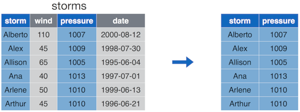
select() keeps only the desired columns of the original dataset.
Note that the list of columns–data variable names–are written
without quotes, exactly as if these were workspace variable names.
Remember, in base-R you need to
quote data variable names as c("storm", "pressure").
This is refered to as non-standard evaluation (see Section 13.7). It
makes the code easier to write and read, but certain tasks, such as
indirect variable
names, are harder to use.
This function is equivalent to the base-R functionality of extracting the columns:
However, even in such a simple example is easier to read and write
with select().
The example above used the select() functions as in standard R,
without the pipes. When using the pipe, you should write:
## # A tibble: 6 × 2
##   storm   pressure
##   <chr>      <dbl>
## 1 Alberto     1007
## 2 Alex        1014
## 3 Allison     1005
## 4 Ana         1013
## 5 Arlene      1015
## 6 Arthur      1010
You can read it as a recipe: a) take the “storms” data; and b) select only columns storm and pressure.
This way of writing code is even simpler than select(storms, storm, pressure) as now it is easier to distinguish between data (storms)
and column names (storm and pressure).
select() is often a good way to start your analysis to make the
dataset, printing, and computer memory requirements more manageable.
It also includes a number of “helper functions” to make it easier to
select certain columns and remove others.
13.3.2 Filter
The filter() operation allows you to choose and extract rows of interest from your data frame (contrasted with select() which extracts columns).
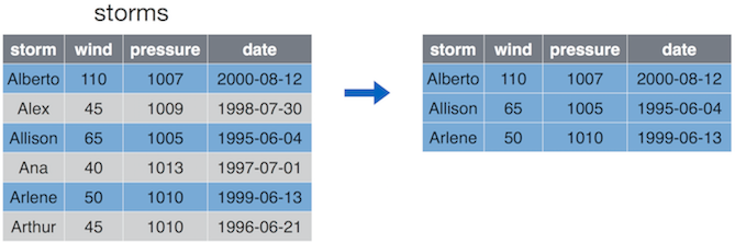
Filter only keeps the rows (observations) that correspond to certain condition. Here we only keep storms where wind is at least 50.
The filter() function takes in the data frame to filter, followed by
a comma-separated list of conditions. Only those rows that satisfy
all these conditions are kept in. For instance, if you write
then you only keep storms where wind is at least 50 and pressure is less than 1000. (We do not have any such storms in the example data here.)
Note again that column names are written without quotation marks!
This function is equivalent to base-R extraction of the rows:
It is much easier to use filter() than the base-R row extraction
when the number of conditions is large.
13.3.3 Mutate
mutate() is the “compute” operation–it allows to create additional
columns in your data frame and modify the existing ones.
## Add `ratio` column that is ratio between pressure and wind
storms %>%
   mutate(ratio = pressure/wind)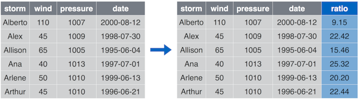
Mutate can create new columns. Here we create a column ratio that is computed as pressure/wind.
The mutate() function takes the original data frame as the first
argument, in the example above, it is fed in through the pipe %>%.
The other arguments are named expressions to calculate, above it is to
compute pressure/wind, and to call the result ratio.
The name = expression syntax it uses is similar that you can use to create
list elements (using list()) or data frame columns (using
data.frame()).
As the habit for dplyr functions,
the names of the columns in the data frame are used without quotation
marks. This is an important upside of mutate(), compare the code
above with the standard way of working with data frames:
Mutate version is both easier to write and easier to read.
Despite the name, the mutate() function doesn’t actually change the
data frame but creates a new one. If you wish to modify the existing
one, you need to re-assign it to the same name:
If you want to create multiple columns in one go, you can just add more computations to the same mutate (separated by comma):
It is a good idea to split different computations on separate lines for readability.
Exercise 13.2 Take the babynames dataset. Add a new column, “decade” to it, so for instance the year “2004” is converted to decade “2000” and “1933” → “1930”.
Hint: use integer division %/%, see Section
4.4.1.
See the solution
13.3.4 Arrange
The arrange() operation allows you to sort the rows of your data frame by some feature (column value).
 function")
arrange() orders the rows (observations) by certain values. Here by
the wind speed in increasing order.
By default, the arrange() function will sort rows in increasing
order. If you want to reverse the order (sort in decreasing order),
then you can place a minus sign (-) in front of the column name
(e.g., -wind). You can also use the desc() helper function as in
desc(wind) (see Section 13.6).
You can also pass multiple arguments (data variable names) to
arrange(). The first one is used for sorting, and the second one is
used to break the eventual ties when sorting according to the first
argument, and so on.
You can also supply not just plain data variable names but expressions–something computed from the data variables. For instance
will order the data by the pressure-wind ratio (we called it “ratio” above).
Th function in order to sort first by argument_1, then by argument_2, and so on.
Again, as the other dplyr functions,
arrange() doesn’t actually modify the argument data frame—it
returns a new data frame instead.
13.3.5 Summarize
The summarize() function (aka summarise()) will create a new
data frame that contains a certain “summary” of columns. The summary
can be anything that makes a single value out of the multiple elements
in that column:
##   median
## 1   22.5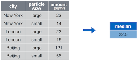
summarize() computes a single value out of a column, here the median
amount.
The summarize() function takes in the data frame to compute on
(through the pipe %>% in the example above) , followed by the rules
about how to compute summary statistics in the form
name = expression.
Note the result: this is a new data frame that contains only a
single row and a single column! In particular, all the original data
is gone, and is replaced by a single summary number (here median).
This may seem counter-intuitive, but it is actually easy to see why
this happens: we request the column amount to be reduced to its
median, a single number. But now summary has no idea how, and if, to
reduce the other columns into a single number. So it just drops the
other columns, unless you explicitly tell it how to reduce those too.
You can use multiple arguments to compute multiple summaries in one go:
pollution %>%
   summarize(
      median = median(amount),  # median value
      mean = mean(amount),  # "average" value
      sum = sum(amount),  # total value
      count = n()  # number of values, see below
)
## median mean sum count
## 1 22.5 42 252 6summarize() looks in many ways similar to mutate(): both compute new
values out of existing columns. But there are two extremely important
differences:
summarize()computes a single value out of columns in each expression.mutate()computes a column out of columns, one value for each row of input.summarize()drops all columns from the original data frame. It only retains a single row (possibly for each group, see see Section 13.5), and only such columns (summaries) that are explicitly requested. In the example above, it will be a data frame of a single row and four columns: median, mean, sum and count.mutate()retains the original data frame with all its rows, possibly replacing some of the columns.
Summary function alone is not particularly useful, you can get similar
results by e.g. median(pollution$amount). But it is an invaluable
tool when working with grouped data (see
Section 13.5)–you can use a single summary()
to get the summary results for all the groups in one go.
Exercise 13.3 Use the babynames dataset. How many names are recorded there over all these years?
See the solution
13.4 Combining dplyr operations
dplyr functions alone are handy. But they turn into an invaluable tool when used as building blocks for more complex data manipulations. It feels almost like building of lego bricks.
dplyr functions are designed to be combined with pipes. Remember: the pipe takes whatever it gets on its left-hand side and feeds it as the first argument to its right-hand side. And this is just what dplyr functions do: they take a data frame in as their first argument (excatly where piped data goes), and they create a new data frame, ready to be fed to another function by pipe. We call such sequence of functions and pipes a “data processing pipeline”.
Think about “babynames” data. Consider the task: how many times, over all these years, was name “Shiva” given to babies? Before you get to coding, you should think how to “divide and conquer” the problem (see Section 9.1). Here we can come up with a simple task list:- filter data to keep only name “Shiva”
- summarize this data set by adding up all counts n
This list translates directly into dplyr functions:
## # A tibble: 1 × 1
##   `sum(n)`
##      <int>
## 1      646
Exercise 13.4
How many times over all these years was name “Shiva” given to girls, and to boys?- write down the task list (not computer code)
- translate it to computer code
See the solution
TBD: remove missings
TBD: assignment and pipelines
TBD: complete this section (dplyr pipelines)
13.5 Grouped Operations
A surprisingly easy and poweful way to extend the functionality is to
allow the functions to work separately by groups–by groups of rows,
defined by certain value(s) of certain column(s).
For example, summarize() we learned above, is not
particularly useful since it just
gives a single summary for a given column, and you can done it
easily with different tools too.
But when we apply summarize() (or
other functions) to grouped data, then it suddenly becomes much
more useful and incredibly powerful.
13.5.1 What are grouped operations
Grouped operations are operations that are done separately for certain groups of rows (groups). The groups are normally defined by values of certain column(s). The data frame is effectively split into several smaller data frames (groups), each corresponding to one value of the grouping column. Thereafter the operations are performed independently on all small data frames, and the results are combined together again.
Let us do an example using Titanic data. If we want to compute the average fare, paid by passengers, we can do it as
## # A tibble: 1 × 1
##   `mean(fare, na.rm = TRUE)`
##                        <dbl>
## 1 33.3mean(titanic$fare, na.rm=TRUE),
and it
tells us that passengers paid £33 in average. But what if we want to
compute this number separately for men and women? We can write the
recipe as
- Take Titanic data
- For each sex value do:
- compute average fare
No problem, it is
easy to do it using filter():
## # A tibble: 1 × 1
##   `mean(fare, na.rm = TRUE)`
##                        <dbl>
## 1 46.2## # A tibble: 1 × 1
## `mean(fare, na.rm = TRUE)`
## <dbl>
## 1 26.2We can see that in average, women paid much more than men for the trip.
This approach is a bit tedious though. But more importantly, it completely fails if the number of groups, here just two (“female” and “male”), is large. Imagine computing yearly averages for monthly data that spans over 100 years, or average delay for each of 200 airplanes in the fleet… While theoretically possible, this approach is too complicated and error-prone to be practical. This is where grouped data comes to play.
dplyr (and many other data analysis frameworks) allow data to be
grouped by values of one or more variables. In the example above,
we used sex as the grouping variable. In dplyr, this can be
achieved with group_by(), for instance:
## # A tibble: 2 × 14
## # Groups:   sex [2]
##   pclass survived name                           sex       age sibsp
##    <dbl>    <dbl> <chr>                          <chr>   <dbl> <dbl>
## 1      1        1 Allen, Miss. Elisabeth Walton  female 29         0
## 2      1        1 Allison, Master. Hudson Trevor male    0.917     1
##   parch ticket  fare cabin   embarked boat   body
##   <dbl> <chr>  <dbl> <chr>   <chr>    <chr> <dbl>
## 1     0 24160   211. B5      S        2        NA
## 2     2 113781  152. C22 C26 S        11       NA
##   home.dest
##   <chr>
## 1 St Louis, MO
## 2 Montreal, PQ / Chesterville, ON
As you can see, the printout of grouped data is almost the same as of the original data. It is still a data frame, the only difference being the note of “Groups: sex [2]” near the top of the output. This tells that it is not just a data frame but a grouped data frame where we have two groups, based on sex.
But importantly, a number of functions now treat grouped data
differently. They perform operations by group–essentially
splitting the dataset into separate datasets for each group,
performing the operation there, and then combining the results back
together. Here is how it works with summarize():
## # A tibble: 2 × 2
##   sex     fare
##   <chr>  <dbl>
## 1 female  46.2
## 2 male    26.2
What summarize() does now is the following (see the figure below):
- The dataset is split into two (or more, if there are more groups) separate partitions based on the grouping variables. Here we only group by sex, and hence we get two separate partitions, one for “male” and one for “female”.
- The following function(s) are applied separately on each partition. Here this means that we compute average fare separately for both men and women. We end up having two data frames: both contain a single row and a single column (see the figure below).
- The partition-specific results results are combined together to the final result. Now we have a data frame with two rows (one for each group) and two columns: one for the mean fare, and the other that tells which group is on which line.
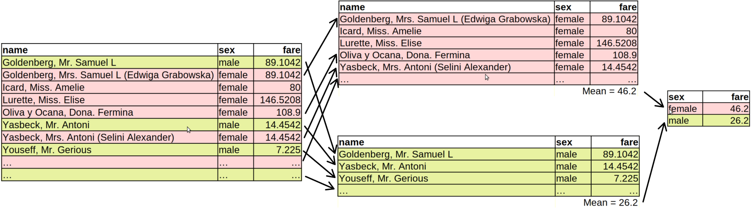
Grouped summary in dplyr: first, the dataset is split by sex into two separate datasets. Thereafter, the summary is computed on each of these partitions separately. Finally, the summary figures are combined again.
Exercise 13.5
Look at different passenger class (pclass) on Titanic.- compute the average and maximum fare
- compute the average and minimum age
Do the results make sense?
See the solution.
In more complex tasks, there are more details regarding how grouped data is processed. In particular, we note following:
Not all functions respect groups by default. One major exception in
arrange(), where you have to tell if you want the data to be ordered within groups byarrange(.by_group = TRUE). In many tasks you actually do not need to arrange by group,rank()will achieve similar results (see Section 13.6.1.3).What happens when you use
summarize()on grouped data is that the result, average fare by sex in the example above, is not grouped any more. Indeed, there is only a single line left for each group, so there is little need to mark that each row is a separate group.But this is not true for all functions. For instance,
mutate()orfilter()will preserve the groups, so when you compute or filter something on grouped data, the results is still grouped data.Sometimes you want your following functions to work on ungrouped data. Certain functions, such as
summarize()does it itself, but if you need to do it explicitly, you can useungroup(). This changes the grouped data frame back to an ungrouped one while leaving everything else unchanged.
We’ll discuss these topics in more details below.
13.5.2 Examples
In this section, we work on a number of examples with grouped data. The purpose of these examples is not just to learn grouped operations, but to practice dplyr functionality more generally. We are using babynames data. We load it with
13.5.2.1 Distinct names
First, how many distinct names are there for years 2002-2006? Here we
can use summarize() and the helper n_distinct() (see Section
13.6.1.4). We can also use the filter()’s
helper between() (see Section 13.6.1.2)
to limit our analysis for this year window:
## # A tibble: 1 × 1
##   `n_distinct(name)`
##                <int>
## 1              44940
So the dataset contains 44,940 distinct names given in these 5
years. But what about the number of distinct names for each year?
This means we need to split data by individual years and do the
computations for each year separately. This is exactly the task that
group_by() is designed for:
babynames %>%
   filter(between(year, 2002, 2006)) %>%
   group_by(year) %>%  # group by year
   summarize(n_distinct(name))  # compute # of distinct names
## # A tibble: 5 × 2
## year `n_distinct(name)`
## <dbl> <int>
## 1 2002 28279
## 2 2003 28886
## 3 2004 29501
## 4 2005 30153
## 5 2006 31624group_by(year) makes dplyr to do the same computations separately
for each year. Here the computations is just what happens inside
summarize()–finding the number of distinct names.
We see that the number fluctuates
around 30,000. This is an incredibly simple way to do a number of
similar computations in a pipeline!
We can repeat the task, but now do it separately for each year and
sex. This is super easy, as group_by() allows to use two grouping
variables:
babynames %>%
   filter(between(year, 2002, 2006)) %>%
   group_by(year, sex) %>%  # group by both year and sex
   summarize(n_distinct(name))
## # A tibble: 10 × 3
## # Groups: year [5]
## year sex `n_distinct(name)`
## <dbl> <chr> <int>
## 1 2002 F 18081
## 2 2002 M 12482
## 3 2003 F 18430
## 4 2003 M 12753
## 5 2004 F 18826
## 6 2004 M 13220
## 7 2005 F 19182
## 8 2005 M 13364
## 9 2006 F 20050
## 10 2006 M 14032Now the groups are defined separately for each unique year-sex combination. We see that there are almost 50% more girls’ names than boys’ names.
Exercise 13.6
Take the complete babynames data, from 1880 to 2017.Compute the number of distinct names for every single year. Print the first few lines of the result.
Find top three years where there were there given most distinct baby names?
Hint: the result of
summarize()is a data frame. You can use the other dplyr operations on that data frame.
See the solution
13.5.2.2 Arranging by group
Ordering observations by group is somewhat special, as this must be
requested separately by the .by_group = TRUE argument of
arrange(). This helps us to find the most popular names for each
year:
babynames %>%
   filter(between(year, 2002, 2006)) %>%
   group_by(year) %>%
   arrange(desc(n), .by_group = TRUE) %>%
   summarize(name = name[1])
## # A tibble: 5 × 2
## year name
## <dbl> <chr>
## 1 2002 Jacob
## 2 2003 Jacob
## 3 2004 Jacob
## 4 2005 Jacob
## 5 2006 JacobHere we group the data by year, and then request it to be arrange, in
the descending order, by n, the count. We tell arrange() to
respect groups and do the ordering separately for each year.
Finally, we summarize by picking the first name from the names for each year. As we ordered it in a descending order, the first name is the most popular one. Hence we get a table of the most popular names for each year. As we can see, it is Jacob for all these years.
Exercise 13.7 Find the most popular boy and girl name for each of these years.
See the solution
An alternative to arranging by group is to use rank(). rank()
behaves in many ways in a similar fashion as arrange(), just it does
not actually change the order, it just tells at which place the
current line would be. For instance,
## [1] 3 1 2tells us that the 1st element (13) should be in the 3rd place, 2nd
element (11)
in the 1st place, and 3rd element (12) in the 2nd place, if we arrange
these numbers in an ascending order. Now we can use rank(desc(n))
in order to tell at which place is a given name, if put in a
descending order. And hence filter(rank(desc(n)) == 1) is the most
popular name. So we can achieve the above with
## # A tibble: 5 × 5
## # Groups:   year [5]
##    year sex   name      n   prop
##   <dbl> <chr> <chr> <int>  <dbl>
## 1  2002 M     Jacob 30568 0.0148
## 2  2003 M     Jacob 29630 0.0141
## 3  2004 M     Jacob 27879 0.0132
## 4  2005 M     Jacob 25830 0.0121
## 5  2006 M     Jacob 24841 0.0113
Exercise 13.8 Find three most popular names for each of these years.
See the solution
13.5.2.3 Most popular names
It is easy to find the most popular name, in terms of largest n:
## # A tibble: 1 × 5
##    year sex   name      n   prop
##   <dbl> <chr> <chr> <int>  <dbl>
## 1  1947 F     Linda 99686 0.0548
This is “Linda” in year 1947. However, it is a very specific way of saying “most popular”. It is not the most popular over time, but the most popular in any given year and sex combination. If we want to find which name has been given most times over all these years and all genders, we have to add n for all names:
## # A tibble: 5 × 2
##   name          n
##   <chr>     <int>
## 1 James   5173828
## 2 John    5137142
## 3 Mary    4138360
## 4 Michael 4372536
## 5 Robert  4834915
We may want the arrange the results by n, currently they are listed alphabetically.
What we do here is the following:- We want to add the counts each name has been used, hence we
summarize
n = sum(n). - However, this should be done separately for each name. This is why we group by name in the line above.
- Finally, we only preserve the the five most popular names.
Exercise 13.9 Find 10 most popular girl names given after year 2000. Order these by popularity!
See the solution
Exercise 13.10 Find the most popular name for each decade from 1880 onward.
Hint: use integer division %/% to compute decade, see Section
4.4.1.
You need to find how many times the name was given through the decade!
See the solution
The previous examples discussed asked questions about which names
had given popularity, now we discuss what is popularity of given
names. This requires us to compute and store the popularity rank
using mutate(). For instance, let’s find at which place was name
“Mei” among girls after year 2000:
babynames %>%
   filter(sex == "F") %>%
   filter(year > 2000) %>%
   group_by(year) %>%
   mutate(k = rank(desc(n))) %>%
   filter(name == "Mei")
## # A tibble: 17 × 6
## # Groups: year [17]
## year sex name n prop k
## <dbl> <chr> <chr> <int> <dbl> <dbl>
## 1 2001 F Mei 29 0.0000146 4261
## 2 2002 F Mei 30 0.0000152 4227
## 3 2003 F Mei 45 0.0000224 3260
## 4 2004 F Mei 35 0.0000174 4038.
## 5 2005 F Mei 32 0.0000158 4315
## 6 2006 F Mei 47 0.0000225 3438
## 7 2007 F Mei 48 0.0000227 3452.
## 8 2008 F Mei 32 0.0000154 4698.
## 9 2009 F Mei 46 0.0000227 3532.
## 10 2010 F Mei 33 0.0000168 4440
## 11 2011 F Mei 39 0.0000201 3874.
## 12 2012 F Mei 39 0.0000201 3944.
## 13 2013 F Mei 46 0.0000239 3430.
## 14 2014 F Mei 49 0.0000251 3292.
## 15 2015 F Mei 44 0.0000226 3553
## 16 2016 F Mei 54 0.000028 3066.
## 17 2017 F Mei 52 0.0000277 3096.Exercise 13.11 Repeat the above. But now compute popularity of “Mei” by decade from 1880 onward.
Hint: use integer division %/% to compute decade, see Section
4.4.1.
You need to find how many times was the name give through the decade!
See the solution
13.5.2.4 A few complex examples
Pipelines can be used for quite complex tasks. Here is a pipeline that answers the following question:
Which names have been among the 10 most popular names for the longest consecutive time period for both boys and girls? And when was that time period?
babynames %>%
   group_by(sex, year) %>%
   filter(rank(desc(n)) <= 10) %>%
   group_by(sex, name) %>%
   arrange(year, .by_group=TRUE) %>%
   mutate(difference = year - lag(year)) %>%
   mutate(difference = ifelse(is.na(difference), 0, difference)) %>%
   mutate(gap = difference > 1) %>%  # there was a year outside of top-10
   mutate(spell = cumsum(gap)) %>%  # separate indicator for each spell
   group_by(sex, name, spell) %>%
   summarize(length = n(), start = first(year), end=last(year)) %>%
   group_by(sex, name) %>%
   filter(rank(desc(length)) == 1) %>%  # pick the longest spell
   arrange(desc(length)) %>%
   head(10)  # just print the first 10
## # A tibble: 10 × 6
## # Groups: sex, name [10]
## sex name spell length start end
## <chr> <chr> <int> <int> <dbl> <dbl>
## 1 M James 0 113 1880 1992
## 2 M John 0 107 1880 1986
## 3 M Robert 2 102 1888 1989
## 4 M William 0 96 1880 1975
## 5 F Mary 0 92 1880 1971
## 6 M Charles 0 75 1880 1954
## 7 M Michael 0 74 1943 2016
## 8 F Margaret 0 60 1880 1939
## 9 M George 0 58 1880 1937
## 10 M David 0 57 1936 1992We do not provide any explanation here, but you can figure it out, line-by-line. However, this also indicates a limit of pipelines: long and complex pipelines are not easy and intuitive any more, and breaking these up into shorter blocks may be preferable.
13.6 More advanced dplyr usage
13.6.1 Helper functions
dplyr functions support a large number of “helper” functions and other supporting language constructs. Below we discuss some of those.
13.6.1.1 Selecting variables
This includes select() but also other
functions that support variable selection.
var1:var2: select range, all variables fromvar1tovar2in the order as they are in data frame.!var1: select everything, exceptvar1!(var1:var2): select everything, except variables in this range.new = old: select variableoldbut rename it tonewstarts_with(),ends_with(),contains(): select variables, name of which begins with, ends with, or contains a certain text pattern.num_range("x", 1:3): select variablesx1,x2,x3c()can combine multiple items for selection
see more with ?select_helpers.
Here are a few examples:
## # A tibble: 2 × 4
##    year sex   name      n
##   <dbl> <chr> <chr> <int>
## 1  1880 F     Mary   7065
## 2 1880 F Anna 2604## # A tibble: 2 × 4
## year sex name n
## <dbl> <chr> <chr> <int>
## 1 1880 F Mary 7065
## 2 1880 F Anna 2604babynames %>%
## rename n to count, include name too
select(c(count=n, name)) %>%
## note that the output is in the selected order
head(2)## # A tibble: 2 × 2
## count name
## <int> <chr>
## 1 7065 Mary
## 2 2604 Anna13.6.1.2 Filtering observations
Useful helper functions for filter() include
between() is a way to select values between two boundaries.
Here are the entries for name “Shiva” between 2002 and 2003 (note:
both these years are included!):
## # A tibble: 4 × 5
##    year sex   name      n       prop
##   <dbl> <chr> <chr> <int>      <dbl>
## 1  2002 F     Shiva     6 0.00000304
## 2  2002 M     Shiva    22 0.0000106
## 3  2003 F     Shiva     5 0.00000249
## 4  2003 M     Shiva    17 0.0000081
rank() filters based on ranking of values. The idea of ranking is
basically ordering–however, we do not actually order the values,
rank just tells at which place the value will be if ordered.
For instance, find the most popular names for girls in 2003:
## # A tibble: 3 × 5
##    year sex   name        n   prop
##   <dbl> <chr> <chr>   <int>  <dbl>
## 1  2003 F     Emily   25688 0.0128
## 2  2003 F     Emma    22704 0.0113
## 3 2003 F Madison 20197 0.0101Rank has a few extra arguments regarding how to break ties, and what
to do with NA-s. See ?rank.
See also row_number() in Computing values
below.
A very useful function (or actually an operator) is
%in% (see Section 10.4). It
tests if values are in a set (both values and the set can be arbitrary
vectors). It returns a logical vector, where TRUE marks that the
element is in the set and FALSE marks that it is not. For instance
## [1] FALSE TRUE TRUEtells us that “a” is not in the set but “b” and “c” are. This is equivalent to a series of equal-to expressions
## [1] FALSE TRUE TRUEbut much more compact.
This is a very useful tool for filtering, as it allows to include any of multiple values. For instance, let’s filter names “Ocean”, “Sea”, “River”, “Lake” for year 2003:
## # A tibble: 6 × 5
##    year sex   name      n       prop
##   <dbl> <chr> <chr> <int>      <dbl>
## 1  2003 F     River    72 0.0000359
## 2  2003 F     Ocean    66 0.0000329
## 3  2003 F     Lake      7 0.00000349
## 4  2003 M     River   388 0.000185
## 5  2003 M     Ocean    69 0.0000329
## 6  2003 M     Lake     61 0.0000290
We can see that there were a number of babies names “Ocean”, “River” and “Lake”, but no “Sea”-s in 2003.31
%in% also works with numbers.
Exercise 13.12 How many names “Sea” and “Creek” were given in year 1980, 1985, 1990, 1995 and 2000?
See the solution
13.6.1.3 Computing values
row_number()is the current row number, possibly within the group. If the data is arranged somehow, then it is similar torank()(see below).rank()is the rank in ascending (or descending) order of a variable, possibly withing a group. Normally,rank()orders in an ascending order, userank(desc(variable))if you want a descending order. Rank is not well-defined if there are ties in data, in that case you may want to specify the additional argumentties.method. See more with?rank.
For instance, compute the rank of name “Shiva” for boys in year 2003:
babynames %>%
   filter(year == 2003,
          sex == "M") %>%
   mutate(rank = rank(desc(n))) %>%
                           # in descending order
   filter(name == "Shiva")
## # A tibble: 1 × 6
## year sex name n prop rank
## <dbl> <chr> <chr> <int> <dbl> <dbl>
## 1 2003 M Shiva 17 0.0000081 4710.lag()gives the value of previous observation, i.e. the value of the same variable in the line above. If it is the first line (possibly within a group), then it returnsNA. For instance, we can compare the current circumference with the previous, and compute growth of orange trees:Orange %>% filter(Tree == 1) %>% # look only for tree 1 for simplicity mutate(prev = lag(circumference), # previous circumference growth = circumference - prev) %>% # difference b/w current and previous head()## Tree age circumference prev growth ## 1 1 118 30 NA NA ## 2 1 484 58 30 28 ## 3 1 664 87 58 29 ## 4 1 1004 115 87 28 ## 5 1 1231 120 115 5 ## 6 1 1372 142 120 22Note that the first prev is
NA, because there is no previous value to pick it from.lag()is group-aware if data is grouped, so it does not cross group boundaries. For instance, it does not pick the last circumference of tree 1 and the previous value for tree 2.
13.6.1.4 Summary functions
count()is a shortcut ofgroup_by() %>% summarize(n = n()). This is useful to count distinct values by group. For instance, we can count, how many times each name is there in the _babynames_data:
## # A tibble: 6 × 2
##   name          n
##   <chr>     <int>
## 1 Aaban        10
## 2 Aabha         5
## 3 Aabid         2
## 4 Aabir         1
## 5 Aabriella     5
## 6 Aada          1
This must be understood that there are 10 lines (year/sex combination) of “Aaban”, 5 lines of “Aabha” and so on.
n()is the total number of observations, possibly within the groupn_distinct()tells the number of distinct values, potentially within group:
## number of distinct names by sex
babynames %>%
   group_by(sex) %>%
   summarize(names = n_distinct(name))
## # A tibble: 2 × 2
## sex names
## <chr> <int>
## 1 F 67046
## 2 M 40927Exercise 13.13
- Make a frequency table of girls’ name popularity for year 2004–how many names names are there that have been given 5 times? 6 times? And so on.
- Now do a similar table for all names, all times: how many names have been given 5 times over all years and both genders? 6 times? etc.
See the solution
13.6.2 Other functions
13.6.2.2 Distinct
The distinct() operation allows you to extract distinct values (rows) from your data frame—that is, you’ll get one row for each different value in the dataframe (or set of selected columns). This is a useful tool to confirm that you don’t have duplicate observations, which often occurs in messy datasets.
For example (no diagram available):
df <- data.frame(
   x = c(1, 1, 2, 2, 3, 3, 4, 4),  # contains duplicates
   y = 1:8  # does not contain duplicates
)
# Select distinct rows, judging by the `x` column
distinct(df, x)
## x
## 1 1
## 2 2
## 3 3
## 4 4# Select distinct rows, judging by the `x` and `y`columns
distinct(df, x, y) # returns whole table, since no duplicate rows## x y
## 1 1 1
## 2 1 2
## 3 2 3
## 4 2 4
## 5 3 5
## 6 3 6
## 7 4 7
## 8 4 8While this is a simple way to get a unique set of rows, be careful not to lazily remove rows of your data which may be important.
13.6.2.3 pull
pull() is a function that extracts a single variable as a vector.
For instance, if we have a data frame
## x y
## 1 1 a
## 2 2 b
## 3 3 c
## 4 4 dthen
## [1] 1 2 3 4will return x as a vector, not as data frame.
This is sometimes confused with select(), e.g.
##   x
## 1 1
## 2 2
## 3 3
## 4 4will also extract x variable only, but select returns a data frame, not a vector.
This is a very important difference, as your further data processing
steps my need x either in a vector or a data frame form. Hence you
need to pick either pull() or select(), depending on what kind of
data structure you need later for your data processing.
13.6.2.4 slice
slice() is another option to keep only certain rows of the data
frame, a bit like filter(). However, while filter() uses logical
conditions to decide which rows to keep, slice() uses rown numbers
(numberic indexing).
Here is a small example using the same df we created above for
pull() (Section 13.6.2.3):
##   x y
## 1 1 a
## 2 2 b
## 3 3 c## x y
## 1 1 a
## 2 4 d## x y
## 1 3 c
## 2 4 d13.7 Non-Standard Evaluation
13.7.1 Data masking
One of the features that makes dplyr such a clean and attractive way
to write code is that inside of each function, you’ve been able to
write column variable names without quotes.
This is called data masking, dplyr lets you to use
data variable names in a similar way as workspace variable names.
Consider this example:
##   mean(x)
## 1      12
Note how mean(x) selects the data variable “x” (11-13), not the
workspace variable “x” (1-3). This is data masking in action.
But be aware that being able to use data variable names without quotes, although convenient, is also more ambiguous. R has to do some guesswork that is usually, but not always, correct. Remember–using the base-R tools you would compute the mean as
## [1] 12This is unambiguous–df$x can only refer to data variables “x”, not
the workspace variable with the same name.
13.7.2 Indirect variable names and dplyr
Writing data variable names without quotes is an easy and convenient way of doing things if we know the variable names when writing the code (see Section 12.3.1). But sometimes we do not know what is the variable we need to work with, e.g. when we let the user to decide what exactly to compute. In such a case we normally store the variable name in another variable–the name is indirect. However, this may be tricky when using quote-less names with dplyr. Fortunately, there are solutions. Below we use a simple demo data frame
For a number of functions, you can use indirect variable names by
wrapping the name into all_of():
##   x
## 1 1
## 2 2
## 3 3
Exercise 13.14 Here select figured out that col refers to a workspace variable
that has value “x”. But what will happen if the data frame also
contains a variable “col”?
For other functions, you can use the variable .data–this is the
data frame the dplyr functions are working on. .data can be used
with the base-R methods, such as .data[[col]] to access the column,
stored in the workspace variable “col” (see Section
12.3.1). For instance, we can filter cases with
##   x  y
## 1 2 12
and summarize variables as
##   avg
## 1   2
13.8 Cleaning data {cleaning}
TBD: data cleaning using dply
TBD: removing missings and why you only want to remove them in the relevant columns
Resources
- dplyr and pipes: the basics (blog)
- Programming with dplyr
- R for Data Science Ch 5: Data transformation: a good introduction to dplyr
Note that the air pressure in this dataset differs from that on the figure. I haven’t understood how the air pressure on the figure is calculated.↩︎
Remember: the dataset includes only names that were given at least 5 times for the given sex. Hence it is possible that there were up to 4 boy and girl “Sea”-s.↩︎