I Dataset Description
Here is a brief description of the datasets that are used in this book.
I.1 Alcohol disorders
In the book repo: alcohol-disorders.csv.
Share of males and females, suffering from alcohol use disorders (percentage of population). Alcohol dependence is defined by the International Classification of Diseases as the presence of three or more indicators of dependence for at least a month within the previous year. This is given as the age-standardized prevalence which assumes a constant age structure allowing for comparison by sex, country and through time.
IHME, Global Burden of Disease Study (2019) – processed by Our World
in Data.
Dowloaded from OWiD
Variables:
- Entity: country, only Argentina, Kenya, Taiwan, Ukraine and the U.S. are included.
- Code: 3-letter country code
- Year: 2015–2019 (only a subset of the original)
- disordersM: number of cases of alcohol use disorders per 100 people, in males, age-standardized
- disordersF: number of cases of alcohol use disorders per 100 people, in females, age-standardized,
- population: Population (historical estimates),
Example:
## # A tibble: 4 × 6
##   country       Code   Year disordersM disordersF population
##   <chr>         <chr> <dbl>      <dbl>      <dbl>      <dbl>
## 1 United States USA    2016      2.90       1.72   327210208
## 2 Kenya         KEN    2016      0.744      0.655   47894668
## 3 Taiwan        TWN    2019      0.903      0.258   23777742
## 4 Argentina     ARG    2018      3.04       1.17    44413592
I.2 Amazon reviews
Reviews of beauty products from Amazon, a random sample of 20 from a larger dataset. Originally downloaded from https://nijianmo.github.io/amazon/index.html, the originals are in json.
Columns:- date: date of the review
- verified:
- summary: (user provided) summary of the review
- review: user’s review of the product
- rating: 1-5, 1 being the lowest and 5 the highest rating.
Example:
## # A tibble: 2 × 5
##   date       verified summary
##   <date>     <lgl>    <chr>
## 1 2014-07-08 TRUE     Good color don't stay
## 2 2014-03-18 TRUE     Light Weight
##   review
##   <chr>
## 1 Polish chips very easily  Love the color.
## 2 This is a light weight conditioner as described.  It is not deep conditioning if y…
##   rating
##    <dbl>
## 1      2
## 2      3
I.3 Any drinking
In the book repo: alcohol-disorders.csv.
Estimates for alcohol consumption for patterns in 10 randomly selected U.S. counties for 2008 and 2012. The numbers represent prevalence (= drinkers/adult population) of drinking in each county. The data comes from the Drinking-patterns study. at the Institute for Health Metrics and Evaluation website, and was downloaded from healthdata.org. For “any drinking”, drinkers are those who consumed at least one drink of any alcoholic beverage in the past 30 days.
Estimates are provided for males and females separately, as well as both sexes combined.
Columns: * state: name of the state * location: county name. For state level observations it is the same as state * both_sexes_2008, females_2008, males_2008: the corresponding drinking rates for everyone, females and males. It includes years 2008 and 2012.
Example:
## # A tibble: 3 × 8
##   state     location        both_sexes_2008 females_2008 males_2008 both_sexes_2012
##   <chr>     <chr>                     <dbl>        <dbl>      <dbl>           <dbl>
## 1 Wisconsin Marathon County            71.5         67         76.1            68.5
## 2 Kansas    Hodgeman County            47.7         36.9       59              49.3
## 3 Arkansas  Woodruff County            37.6         28.2       47.2            37.6
##   females_2012 males_2012
##          <dbl>      <dbl>
## 1         65.2       71.8
## 2         40.5       58.5
## 3         28.2       47.3
I.4 Babynames
R package babynames contains a dataset babynames. It includes all names, given to babies born in the U.S. between 1880-2017. Only names that were given to at least 5 babies each year for each sex. Data originates from the U.S. Social Security Administration.
You can load it with library(babynames), that loads a single data
frame babynames.
Example:
## # A tibble: 3 × 5
##    year sex   name        n       prop
##   <dbl> <chr> <chr>   <int>      <dbl>
## 1  2017 F     Safiyah    29 0.0000155
## 2  2004 F     Faryn       8 0.00000397
## 3 1931 F Anna 8430 0.00764- year: 1880-2017
- name: the name
- sex: “F” or “M”
- n: how many babies got this name (withing year/sex)
- prop: proportion of babies who got this name in the given year (within year/sex).
I.5 Country-concept similarity
In the book repo: country-concept-similarity.csv.bz2. This dataset shows the similarity between country names and a set of different words, and it is calculated based on texts that were scraped from internet around 2015. The dataset looks like
## # A tibble: 2 × 12
##   country     terrorism nuclear  trade battery  regime volcano  palm    fir  flood
##   <chr>           <dbl>   <dbl>  <dbl>   <dbl>   <dbl>   <dbl> <dbl>  <dbl>  <dbl>
## 1 aruba          0.0891  -0.011 0.0504 -0.01   -0.0356   0.166 0.293 0.0965 0.0158
## 2 afghanistan    0.447    0.220 0.109   0.0578  0.180    0.129 0.116 0.129  0.159
##   drought mountain
##     <dbl>    <dbl>
## 1  0.0581    0.107
## 2  0.160     0.161
One can see that “Afghanistan” and “terrorism” are much more similar (similarity 0.447) than e.g. “Afghanistan” and “trade” (similarity 0.109). We do not go into details here about how the similarity is measured, but broadly, it means how frequently are these words used in a similar context as the corresponding country names.
I.7 CS-GO
Dataset about CS-GO (video game) reviews: each line is a review. It is scraped from Steam website by mulhod, see the original repo at GitHub. The dataset is not really documented, but you can guess based on the column names.
Sample:
## # A tibble: 3 × 8
##   rating      nHelpful nFunny nScreenshots date                 hours nGames nReviews
##   <chr>          <dbl>  <dbl>        <dbl> <chr>                <dbl>  <dbl>    <dbl>
## 1 Recommended        4      1           19 Jun 30, 2014, 2:16AM 1888.    131        3
## 2 Recommended        5      0           56 Jan 18, 2014, 3:45AM  283.    127        7
## 3 Recommended 5 1 11 Dec 19, 2013, 9:55PM 1442. 88 1- rating”: Recommended/Not recommended
- nHelpful”: number voted helpful
- nFunny”: number found funny
- nScreenshots”: number of screenshots
- date”: date posted
- hours”: total game hours by the reviewer
- nGames”: number of games
- nReviews”: number of reviews
TBD: anyone knows steam and can help here?
I.8 Diamonds
It is a built-in dataset in ggplot2 library, so it is already loaded when you load the library. It contains price, shape, color and other information for 53940 diamonds. A sample of it looks
## # A tibble: 5 × 10
##   carat cut       color clarity depth table price     x     y     z
##   <dbl> <ord>     <ord> <ord>   <dbl> <dbl> <int> <dbl> <dbl> <dbl>
## 1  0.23 Very Good E     VVS2     60.6    60   505  3.93  3.99  2.4
## 2  0.9  Very Good H     SI1      63      55  3388  6.12  6.16  3.87
## 3  1.53 Premium   H     SI1      59.5    59 10398  7.53  7.46  4.46
## 4  0.3  Very Good E     SI1      60.6    56   526  4.35  4.37  2.64
## 5 1.34 Premium I VS2 61.8 59 6754 7.07 7.04 4.36carat: mass of diamonds in caracts (ct), 1 ct = 0.2g
cut: cut describes the shape of diamond. There are five different cuts: Ideal is the best and Fair is the worst in these data. Better cuts make diamonds that are more brilliant.
Note: cut is an ordered factor, see Section 21.2.3.
color: There are 7 color levels, J (no color) is the best and D the worst, any color hue is considered not desirable.
clarity: measures the defects in diamonds, IF (internally flawless) is the best, and I1 is the worst.
depth, table: measures of the diamond shape
price: in $
x, y, z: diamond size, mm
I.9 Fatalities
In the book repo: fatalities.csv
The U.S. Traffic fatalities by state in 1980’s. This is a subset of dataset Fatalities in the AER package. Example:
## # A tibble: 4 × 4
##    year state fatal      pop
##   <dbl> <chr> <dbl>    <dbl>
## 1  1982 MN      571 4133009
## 2  1985 MN      608 4192988.
## 3  1987 WA      780 4537997
## 4 1983 WA 698 4305001- year: 1982-1988
- state: only MN, OR, WA
- fatal: total number of traffic fatalities
- pop: population
I.10 Height-weight
In the book repo: height-weight.csv.
Synthetic dataset of five lines to demonstrate certain data properties. Here is the whole dataset, the meaning of columns is obvious:
## # A tibble: 5 × 4
##   sex      age height weight
##   <chr>  <dbl>  <dbl>  <dbl>
## 1 Female    16    173   58.5
## 2 Female    17    165   56.7
## 3 Male      17    170   61.2
## 4 Male      16    163   54.4
## 5 Male      18    170   63.5
I.11 Icecream
It is located in package Ecdat. It contains 30 four-weekly observations of ice cream consumption in 1950s in the U.S. Example:
##     cons income price temp
## 20 0.342     86 0.277   60
## 25 0.309     95 0.282   28
## 22 0.307     87 0.287   40
## 11 0.286 82 0.282 28- cons: consumption of ice cream per head (in pints);
- income: average family income per week (in US Dollars);
- price: price of ice cream (per pint);
- temp: average temperature (in Fahrenheit);
I.12 Ice extent
TBD: an explanatory figure of area/extent
In the book repo: ice-extent.csv.bz2.
National Snow & Ice Data Center (NSIDC) data about sea ice extent and area. Downloaded from U Colorado
A sample of data:
## # A tibble: 5 × 7
##    year month `data-type` region extent  area  time
##   <dbl> <dbl> <chr>       <chr>   <dbl> <dbl> <dbl>
## 1  2020     2 Goddard     N       14.6  13.0  2020.
## 2  2012     2 Goddard     N       14.6  12.7  2012.
## 3  2011     5 Goddard     S       10.1   7.85 2011.
## 4  1983     1 Goddard     S        4.77  3.21 1983.
## 5 2022 7 NRTSI-G S 14.9 11.9 2023.- year
- month: (1-12)
- data-type: looks like the name of the satellite or another info provider
- region: “N” for northern, “S” for southern hemisphere
- extent: sea ice extent, in M km2. Extent is the sea surface area where the ice concentration is at least 15%.
- area: sea ice surface area, M km2
- time: a continuous time variable, made of year and month \(\mathit{time} = \mathit{year} + \mathit{month}/12 - 1/24\). This describes roughly the middle of each month as measured in years.
I.13 Iris
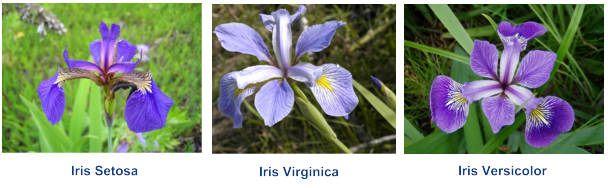
Iris flowers are beautiful. setosa, virginica and versicolor.
Iris dataset is collected by Ronald Fisher 1936. It contains sepal and petal measures of 150 iris flowers of species setosa, versicolor and virginica (50 of each). It is an R built-in dataset and does not even have to be loaded, you can just use it as variable iris, a data frame with 150 rows and 5 columns.
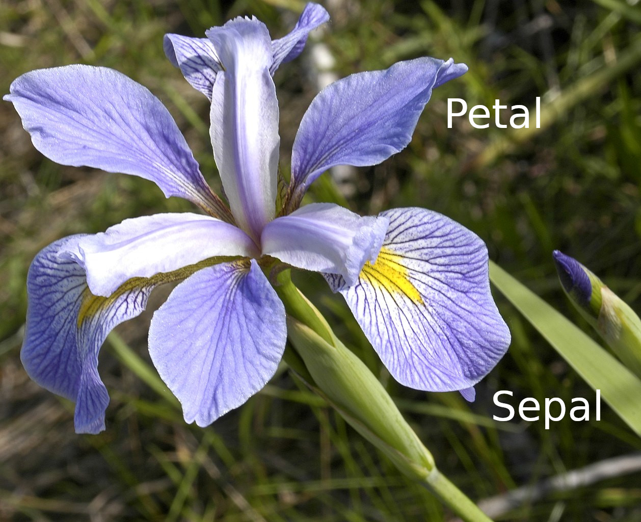
Petals and sepals are parts of the flower (virginica).
- Sepal.Length: sepal length, in cm
- Sepal.Width
- Petal.Length
- Petal.Width
- Species: setosa/versicolor/virginica
A small example of it:
##   Sepal.Length Sepal.Width Petal.Length Petal.Width    Species
## 1          6.0         3.4          4.5         1.6 versicolor
## 2          6.1         2.8          4.7         1.2 versicolor
## 3          7.9         3.8          6.4         2.0  virginica
## 4          6.9         3.1          5.1         2.3  virginica
I.14 Orange tree growth
It is an R built-in dataset, however, as that uses more complex data structures, a copy of it is in repo as a plain csv file: orange-trees.csv
Variables:- Tree: an ordered factor indicating the tree on which the measurement is made. The ordering is according to increasing maximum diameter.
- age: a numeric vector giving the age of the tree (days since 1968/12/31)
- circumference: a numeric vector of trunk circumferences (mm). This is probably “circumference at breast height”, a standard measurement in forestry.
I.15 Storms
In repo as storms.csv.
A tiny version of the storms dataset that is included in dplyr. It contains 6 storms only, and one line per the storm. Used to explain dplyr. Columns:
- storm: storm name
- wind: maximum wind speed (knots)
- pressure: maximum air pressure (mbar). Note: this may be a different day than the date of the maximum wind speed.
- date: date of the maximum wind speed (first date if multiple such dates).
Example:
## # A tibble: 3 × 4
##   storm    wind pressure date
##   <chr>   <dbl>    <dbl> <date>
## 1 Ana        40     1013 1997-07-01
## 2 Arthur     45     1010 1996-06-21
## 3 Allison    65     1005 1995-06-04
I.16 Titanic
In repo as titanic.csv.bz2.
List of RMS Titanic passengers, their name, age and some more data, and whether they survived the shipwreck. It was collected by the investigation committee, and contains most of the passengers on the boat. The dataset is available in various sources, e.g. at kaggle. The variables are
- pclass: Passenger Class (1 = 1st; 2 = 2nd; 3 = 3rd)
- survived: Survival (0 = No; 1 = Yes)
- name: Name
- sex: Sex
- age: Age
- sibsp: Number of Siblings/Spouses Aboard
- parch: Number of Parents/Children Aboard
- ticket: Ticket Number
- fare: Passenger Fare
- cabin: Cabin
- embarked: Port of Embarkation (C = Cherbourg; Q = Queenstown; S = Southampton)
- boat: Lifeboat code (if survived)
- body: Body number (if did not survive and body was recovered)
- home.dest: The home/final destination of passenger
A small example of it:
| pclass | survived | name | sex | age | sibsp | parch | ticket | fare | cabin | embarked | boat | body | home.dest |
|---|---|---|---|---|---|---|---|---|---|---|---|---|---|
| 2 | 1 | West, Miss. Barbara J | female | 0.9167 | 1 | 2 | C.A. 34651 | 27.7500 | NA | S | 10 | NA | Bournmouth, England |
| 3 | 0 | Johansson, Mr. Nils | male | 29.0000 | 0 | 0 | 347467 | 7.8542 | NA | S | NA | NA | NA |
| 1 | 1 | Leader, Dr. Alice (Farnham) | female | 49.0000 | 0 | 0 | 17465 | 25.9292 | D17 | S | 8 | NA | New York, NY |
| 3 | 0 | Perkin, Mr. John Henry | male | 22.0000 | 0 | 0 | A/5 21174 | 7.2500 | NA | S | NA | NA | NA |
I.17 Tomato growth at different temperature
Synthetic data about three tomato plants, growing at different temperature. Used to demonstrate continuous and discrete values for plotting.
Columns:- plant: plant id, A, B, or C
- age: in months
- temperature: deg C
- size: cm
Obviously, the units do not really matter for this toy dataset. Example:
## # A tibble: 4 × 4
##   plant   age temperature  size
##   <chr> <dbl>       <dbl> <dbl>
## 1 A         3          15    80
## 2 B         2          21    70
## 3 C         1          25    60
## 4 C         3          18    92
I.18 Ukraine’s regional population
In repo as ukraine-oblasts-population.csv. Copied from the Wikipedia table 2024-03-03. Population as of 2015.
Example:
## # A tibble: 3 × 4
##   Prefecture            Population `Urban population` `Rural population`
##   <chr>                      <dbl>              <dbl>              <dbl>
## 1 Donetsk Oblast           4387702            3973317             414385
## 2 Dnipropetrovsk Oblast    3258705            2724872             533833
## 3 Kyiv                     2900920            2900920                 NA
The variables are self-explanatory.
I.19 Ukraine with regions
In repo as ukraine-with-regions_1530.geojson. The national borders and regional (oblast) borders of Ukraine in geojson format. Provided by Cartography Vectors.
The map:library(sf)
library(ggplot2)
map <- read_sf("data/ukraine-with-regions_1530.geojson")
ggplot(map) +
geom_sf()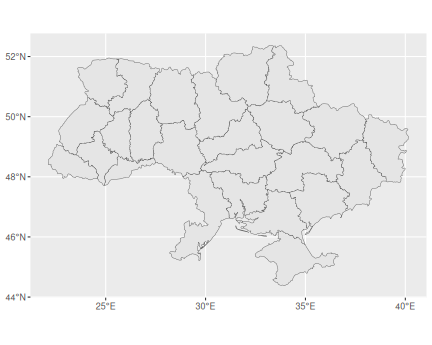
National and regional (oblast) borders of Ukraine. Provided by Cartography Vectors.
I.20 US States
R has multiple small datasets about the US states. They are built-in variables, so you do not need to do anything special to load these. Examples:
## [1] "Alabama" "Alaska" "Arizona" "Arkansas" "California"## [1] "AL" "AK" "AZ" "AR" "CA"Importantly, all these vectors contain data in the same order, so you can use names to find the value for the corresponding state.
I.21 Yin-yang
In repo as yinyang.csv.bz2.
An artificial dataset to demonstrate decision boundary for various classification methods.
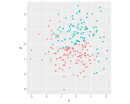
Columns:
- x, y: coordinates
- c: 0/1, color
Example data:
## # A tibble: 3 × 3
##        x      y c
##    <dbl>  <dbl> <fct>
## 1 -1.63   0.584 0
## 2  0.624 -0.113 0
## 3 -0.688  1.74  1
The scatterplot with c marked as color at right.