Chapter 1 Setting up your computer
Through this course we’ll be using a variety of different software programs to write, manage, and execute the code that we write. Unfortunately, one of the most frustrating and confusing barriers to working with code is simply getting your machine properly set up and to understand how the new software works. And you cannot even start before you have got the necessary tools up and running! This chapter aims to provide sufficient information for setting up your machine and troubleshooting the process. All the tools we use are free to use, and they work on all major platforms, including linux, mac and windows.
Through this book you’ll need to two major software packages:
R: a popular programming language for working with data. This is the primary programming language used throughout this book. “Installing R” actually means installing tools that will let your computer understand and run R code.
RStudio: A graphical editor (IDE or Integrated Development Environment) for writing and running R code. This will soon become our primary development application. Strictly speaking, RStudio is not necessary, you can perfectly work with R without it, but it simplifies the work quite a bit. Throughout the book we assume you are using RStudio.
Next we explain these programs in mode detail.
1.1 R Language
The primary programming language you will use throughout this book is called R. It’s a powerful programming language that is designed for statistics and for working with data. See Section 4 for a more in-depth introduction to the language.
In order to use R programs on your computer, you need to install the R Interpreter on your machine. This is a piece of software that is able to “read” code written in R and use that code to control your computer. Such controlling is called “programming”.
The easiest way to install R is to download it from the Comprehensive R Archive Network (CRAN) at https://cran.r-project.org/. Click on the appropriate link for your operating system in order to find a link to the installer.
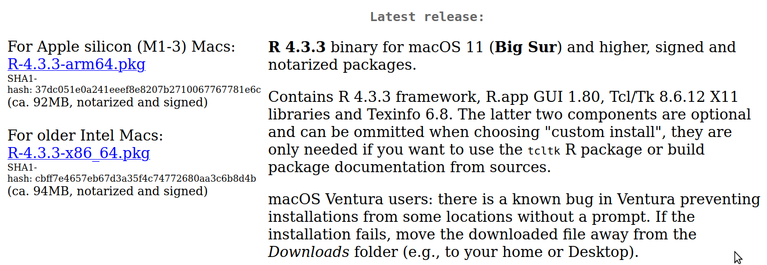
Downloading R for Mac. R 4.3.3 was the latest version as of the time
of writing, but you should always get the most recent one.
Download the blue .pkg file that corresponds to your computer cpu
type.
On a Mac, you’re looking for the
.pkgfile—get the latest version supported by your computer. You also need to use either intel or Apple silicon (M1/M2/…, listed as arm64.pkg) version, depending on your computer type. (If you are not sure, you can find it using “About this mac” in the Apple menu.)To ensure smooth programming with R and RStudio on macOS, you will need to download and install Xquartz. This application supports R functions that were removed in later macOS versions and is essential for using R in the terminal. Note that before macOS 10.8, Xquartz was included by default, so if you have an older macOS then it may already be installed. But you may still check.
- On Windows, follow the link to the
basesubdirectory (or follow the link to “install R for the first time”), then click the link to download the latest version of R (the link titled Download R-4.3.3 for Windows as of the time of this writing). This will download the.exeinstaller, you will need to double-click on it to install the software. Accept the default options, unless you know better. - There are binary versions for popular linux distributions, including ChromeOS. Many distros also include R through they package managers.
1.2 RStudio
While you are able to execute R scripts with just the R app you downloaded above, RStudio provides a much simpler and more polished way to work with the R language. RStudio is described in more detail in Section 1.3.

A selection of different installers on the RStudio download page.
To install the RStudio program, you first need to install R (see above). Thereafter select the installer for your operating system from the RStudio downloads page. Make sure to download the free desktop version, and the correct version for your OS.
The dowload page may suggest to download the windows version, so scroll down and pic another option if you use mac/linux.
Currently (Jan 2025), the most recent RStudio for Mac requires MacOS 12 or later. If you are using an older version of MacOS, you need to download a previous version, see the link under the download button.
Once the download completes, double-click on the .exe or .dmg file
to run the installer. Accept the default options and the default R
installation if asked. Now
you should be prepared to use RStudio.
1.3 A closer look at RStudio
The primary way to use R in this course is through RStudio (see below). It is an open-source integrated development environment (IDE) that provides an informative user interface for interacting with the R interpreter. IDEs are glorified text editors that provide various other handy tools for programming. For instance, RStudio let’s you to edit your program, colors your code in a way to make understanding it easier (syntax coloring), allows you to execute it with a simple keypress, explore data and workspace variables, your command history, install packages, and much more.
1.3.1 Rstudio layout

RStudio’s default user interface. Red texts are annotations.
When you open RStudio (either by searching for it, or double-clicking on a desktop icon), you’ll see an interface that looks something like on the figure here. By default, RStudio interface consists of 4 panes–small windows for different tasks (you can customize this layout if you wish):
Console: The bottom-left pane is a console where you can directly enter and execute the R commands.
Normally you use console for quick computations and short sequences of 1-2 lines of code. Longer blocks of code is usually easier to write as scripts or rmarkdown.
Script: The top-left pane is a text editor for writing R code, markdown, and other files. It contains a plethora of tools to work with R (and some other) code, including syntax coloring (coloring code according the its function), “auto-complete” and formating text, and to execute your code easily. Note that this pane is hidden if there are no open scripts; select File → New File → R Script from the menu to create a new script or File → New File → R Markdown to create a new rmarkdown file (see Section 3.4).
Environment: The top-right pane displays information about the current R environment (workspace)—specifically, information that you have stored inside of workspace variables (see Section 4.3 below). In the example in RStudio script window, the value
201is stored in a variable calledx. You’ll often create dozens of variables within your code, and the Environment pane helps you keep track of which values you have stored in what variables.Plots, packages, help, etc.: The bottom right pane contains multiple tabs for accessing various information about your files and code. When you create visualizations, those plots will also be in that pane. This is also where you can access the documentation. If you have a question about how something in R works, this is a good place to start!
Note, you can use the small spaces between the panes to adjust the
size of each area to your liking. You can also use menu options to
reorganize the panes if you wish. The most useful tools
are focusing and zooming. Focusing means moving your
cursor and input into a particular pane, e.g. Ctrl + 1 makes
the script pane active and Ctrl + 2 makes console pane active.
Using keyboard shortcuts to move your focus is much faster than
grabbing the mouse.
Zooming is a bit similar to focus, just it also hides the other
panes and makes the zoomed on of full size.
Ctrl + Shift + 1 zooms to script, Ctrl + Shift + 2 zooms
to console, and Ctrl + Shift + 0 restores the original 4-pane view. Zooming to
individual panes is very useful if you are working on a small screen.
See the View → Panes
menu and options therein, the menus also list
the keyboard shortcuts.
See Section J for more information.