Chapter 3 Markdown and rmarkdown
When you do coding then you normally write, well, code. Code (computer program) is just list of computer instructions, written underneath each other, line-by-line. It is written to be “run” on computers, and it is designed to be “understandable” for computers. However, in this course we expect you to write not just code for computers, but also explanations for humans. Unfortunately, computer programs are not well-suited for messaging to humans. This is why we use literal programming, a type of programming where you will mix computer code (to be read by computers) with normal text (to be read by humans). We do this using rmarkdown documents. Rmarkdown is made of two things: first, “R” is R, the programming language we’ll use in this course; and second, “markdown” is a special language to write structured text. Next, we’ll discuss markdown and thereafter rmarkdown; R is introduced in Section 4.
3.1 What is markdown
Markdown is a language to create text documents. You are probably familiar with modern text processors, such as Google Docs or Microsoft Word. Such word processors allow you to create beautiful text that may contain images, use multiple fonts and be rendered in multiple columns.
Markdown is not like this. Not at all. But it can create beautiful text too,
although its capabilities are rather limited. Also, it is not a text
processor.
Markdown is a markup language. So it is a language that
has special codes for formatting text. When you write markdown, you
cannot just create bold text, instead you have to include the
formatting codes around the text you want to be bold (here double
asterisks, as in **bold text**). And then we have to render it
into something, e.g. into html,
where the formatting codes are transformed into the
corresponding format, like double asterisks are transformed
into bold font.
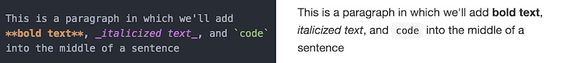
Markdown text formatting. At left, the text in a markdown-aware text editor (using dark theme). You can see how bold and italic are marked using the corresponding symbols. This is how you write markdown. At right, the same text rendered as html. The symbols are replaced by the corresponding style. This is normally the desired final form of the text as written at left.
Why do we need such language that may feel like the text processing tools of 1980-s? There are several reasons. It is true that modern word processors are currently the dominating way to create documents. But they are not good tools to create all sorts of documents. Here are a few reasons why people are using markup languages, such as markdown:
- Markdown does not require dedicated word processors. You can edit markdown documents in every text editor (such as RStudio). The file format is plain ASCII text, the simplest way to store text. So every programmer can use their favorite editors to write documents.
- Markdown can be integrated into various simple document processing environments, such as discord chat or Github documents.
- Markdown is easy to write and learn. There are other markup languages, such as HTML and LaTeX that are much more powerful, but also much more complex.
- Markdown formatting codes are visible. So for instance, you can
use both italics and bold, typed as
_italics_ and **bold**. Now if your cursor is on the space before_and_, you can immediately tell that this space is not italic–it is outside of the italic formatting codes (underscores). This avoids nasty surprises in text processors where you start writing and discover that the text is formatted in an unexpected way. - Word processor file formats are quite complicated. If you want to generate a word processor document not by typing the text manually but through a computer program, you find this to be a formidable task. And this is exactly what we will do using rmarkdown below.
- Because word processor file formats are complicated, they are not easy to combine with version control systems, such as git. Word processors include their own revision controls, but these are fairly limited and do not integrate with dedicated systems like git that are typically used for larger projects.
So Markdown provides a simple way to describe the desired formatting of text documents while leaving rendering for other software. Rendering means transforming markdown text into the final format, such as HTML or pdf, that actually displays the formatting in desired way (instead of format codes). So in markdown you do not create layout, instead of that you tell what kind of layout you want. In fact, this book is written using markdown (with some help of HTML)! With only a small handful of options, markdown allows you to format to your text (like bold and italics), and well define structure of the document (such as headers and bullet-points).
There are many programs and services that support the markdown, including GitHub, Slack, discord, teams, and StackOverflow (though the syntax and capabilities vary somwhat across programs). In this chapter, we’ll learn the basic markdown syntax, how to use it to produce readable documents, and how to combine it with R code.
3.2 The first taste of markdown
Markdown is a markup language that is used to format and structure text. It is a kind of “code” that you write in order to annotate plain text: it lets the computer know that “this text is bold”, “this text is a heading”, etc. Compared to other markup languages, Markdown is easy to write and easy to read. In my opinion, it is much easier that what normal word processors offer, and hence I am sometimes using markdown syntax even in contexts that do not support markdown, such as Google docs. And because markdown is simple to include, it’s often used for formatting in web forums and services (like Wikipedia or Discord). As a programmer, you’ll use Markdown to create documentation and other supplementary materials that help explain your projects, rmarkdown (see Section 3.4) is also a good way to write reports.
The basic markdown workflow to compose documents includes both writing and rendering. This differs from the modern word processors, where these two elements are combined into a single one: if you insert a bold letter into your document, you’ll immediately see that it is bold. In markdown, you need to first write the letter with bold markers, and thereafter to render it into something (e.g. html) that can actually display it as bold. These two steps are separated.
3.2.1 Markdown in RStudio
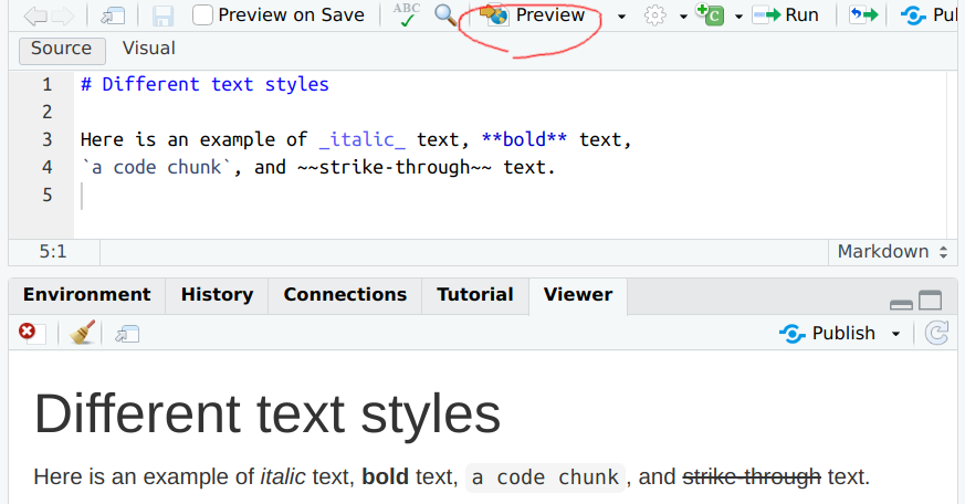
Markdown text (above) and the rendered output (below) in RStudio. The Preview button is highlighted in red.
You can create a new markdown file in RStudio through the menu File → New File → Markdown File. This opens an empty document where you can experiment with the formatting examples below.
Note that this example shows the rendered markdown in the Viewer window below the source window, by default it will be rendered in a separate window.
When you want to view the rendered version of your markdown document, you need to use a program that converts the Markdown into a formatted document. This is automatically included in RStudio.5 You can render your document using the Preview button (highlighted in red).
Later we will work mostly with rmarkdown files (see Section 3.4) that need to be handled slightly differently.
There are other options for rendering Markdown. Some text editors, such as Visual Studio Code or certain online markdown editors will render it automatically. There are also a browser extension that will render Markdown files. Unfortunately, the rendered result and the syntax may differ slightly, depending on what exact tools are used.
3.2.2 Text Formatting
At its most basic, Markdown is used to declare text formatting
options. You do this by adding special symbols around the text you
wish to “mark”. For example, if you want text to be rendered as
italics, you would surround that text with underscores (_):
you would type _italics_, and the rendering program will
render that text as italics. You can see how this looks in the below example (code on the left, rendered version on the right):
There are several ways you can format text:
| Syntax | Formatting |
|---|---|
_text_ |
italics with underscores (_) |
**text** |
bold using two asterisks (*) |
`text` |
inline code with backticks (`) |
~~text~~ |
~) |
Exercise 3.1 Create a new markdown document and experiment with these formatting tools. Write your text as source and use the preview button to render it, do not use visual mode!
3.3 Markdown syntax
But Markdown isn’t just about adding bold and italics in the middle of text—it also enables you to create split your document in sections with different headers, add bullet lists and chunks of code. Below we discuss how to mark the structure, lists, and last bot not least–images and tables.
3.3.1 Structure
Marking text structure tells the renderer what is this text, and let’s the renderer decide how to display it. As structure, we normally mean various section titles, but also paragraphs, pre-formatted text and other similar features.
Line
breaks
are
ignored.
Paragraphs are separated
by a blank line.

Two spaces at the end of a line leave
a
line
break.
Paragraphs are separated by a blank line. Normal line breaks are ignored, so you can break lines wherever you want.
Line
breaks
are
ignored.
Paragraphs are separated
by a blank line.
Two spaces at the end of a line leave
a
line
break.A dedicated line break can be done by ending the line with double spaces–the second paragraph in this example contains such double-space line ends, these are unfortunately not visible in the image.
> in the beginning of the line:
This is a quote:
A clever man commits no minor blunders
– Goethe
In this example, the > A clever man... is a quote, while the lines
before and after it are not. Quote is normally marked somewhat
differently than the rest of the text. It is widely used in online
forums, where you can quote the text you are replying to.
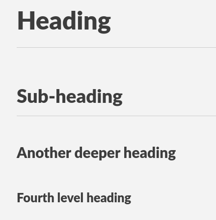
Four different levels of headings, followed by normal text. In this figure, the 4th level heading is scarcely larger than normal text.
Sections are be marked by headings. This example displays four levels of headings:
# Heading
## Sub-heading
### Another deeper heading
#### Fourth level heading

Normal text on a separate line.
These are normally rendered with big and bold font, with the first level headings being the biggest and boldest.
above
below
A horizontal rule can be created with three dashes:
These are useful to separate blocks of text where an new section would be impractical.
One special structure element that we’ll use a lot below are code blocks. In plain markdown, these is not actually code blocks, but just “pre-formatted text”, a piece of text that is displayed as-is, with no additional formatting applied, and where spaces and line breaks are preserved as in the original. Code blocks are rendered using fixed-with font where all letters (including “i” and “m”) are of the same width. This also let’s you use it to display various other things instead of code, such as ascii art or poems.
Code blocks are marked with three backticks before and after the block:library(magick) # install it first
cheatsheet <- image_read_pdf("cheatsheet.pdf")
plot(cheatsheet)```
library(magick)  # install it first
cheatsheet <- image_read_pdf("cheatsheet.pdf")
plot(cheatsheet)
```Here is an example of a code block that contains R code.
Exercise 3.2 Display ascii art in your markdown document as code block. Here is a maple leaf as an example:
     .\^/.
   . |`|/| .
   |\|\|'|/|
.--'-\`|/-''--.
 \`-._\|./.-'/
  >`-._|/.-'<
 '~|/~~|~~\|~'
       |
Hint: you can just search internet for ascii art–there is a plethora of wonderful examples.
3.3.2 Lists
Structured text, such as reports, commonly use lists. There are two types of lists: non-numbered (bullet lists) and numbered lists.
Here are fruits: leave a blank line before you start the list
- apples
- oranges (can use both asterisks and dashes)
- pears
- sublists are indented by 4 spaces
- small pears
- medium pears
The rendered version of the list at left. Both asterists and dases are replaced by bullets.
Bullet lists can be marked with asteristisks (or dashes) at the beginning of the line:
Here are fruits: leave a blank line next

* apples
- oranges (can use both
  asterisks and dashes)
* pears
    - sublists are indented by 4 spaces
    - small pears
    - medium pears
You need to leave one blank line above the list, otherwise it will be not rendered as a list, but just sentences that contain asterisks. You also need to leave one space after the asterisk.
Note that lists can be nested–the nested list must be indented by 4 (four) spaces right of the parent list.
Fruits in priority order:
- mangoes (note the format–number, dot, space)
- oranges
- pears (will be rendered as “3.”)
- sublist (numbering starts from “2”)
- small pears (indented by 4 spaces)
- medium pears
The list at left as rendered. Note that the renderer has fixed the numbering.
Fruits in priority order:

1. mangoes (note the format--number,
   dot, space)
2. oranges
4. pears (will be rendered as "3.")
    2. sublist (numbering starts from "2")
    3. small pears (indented
       by **4** spaces)
    3. medium pears
Markdown normally fixes list numbering, so whatever numbers you put in front of your lines, the result will be “1.”, “2.”, etc… But if you start your numbering from “2.”, the you will get “2.”, “3.”, etc.
As in case of bullet list, you need to leave an empty line above the list, and a space after the number (after the period).
Exercise 3.3 Write a numbered list of cities. Under at least two of one of the cities, write a list of restaurants in that city as a non-numbered sublist.
Feel free to invent!
3.3.3 Text
There are multiple ways to format individual words, or parts of the word.
Underscore marks italics, double asterisks bold, and double tildes striked through text:italic
bold
bold italic
strike through
(There are other ways to achieve these attributes.)
[link text](url). For instance:
Here’s an example
Here's [an example](http://example.com)The link text will be the visible text that you can click on (often rendered blue), and the click will lead you to the url.
3.3.4 Images and tables
More often than not, we want to illustrate our text with images.
Fortunately, this is easy.
Images can be inserted by :

CC BY 2.0 by slava, via Wikimedia Commons
The anatomy of the markdown command is as follows:
!tells markdown to actually display the image in text, not just a clickable link. (Note: the syntax is otherwise the same as for web links.)[]can contain the “alternate text” attribute, the text that the browser renders when it cannot render the image. This may happen if you have got the file path wrong, or if you are using screen reader, a search engine or a web scraper.(image.jpg)contains the actual image, either file name (possibly with a path), or an url. For instance, the same cat image can be displayed straight from wikimedia using.
Note that unlike in R code, the file name must not be quoted! (See Section @ref(file-system-tree.html) for more about how R reads files.)
Another type of commonly used illustration is tables. Tables are somewhat inconvenient to create in markdown, but for small and simple tables, it is OK.6 Here is an example:| fruit | quantity | price |
|---|---|---|
| apples | 3 | 6 |
| oranges | 4 | 8 |
| bananas | 1 | 2 |
|     fruit | quantity | price |
|  -------- | :------: | ----: |
|    apples |        3 |     6 |
|    oranges|        4 | 8|
|bananas|1|2|
The table defines three columns, labeled fruit, quantity and price, separated by vertical bars. The next line, that of dashes, defines the indentation. The first column is lef-justified, quantity-column is centered, and price-column is right-justified.
The first line (apples) is written in a good and clear manner, the oranges-line lacks some spacing, and bananas is written with no spacing at all. However, the renderer ignores spaces and displays all these columns in an equally pleasant manner.
For more thorough lists of Markdown options, see the resources linked below.
Finally, we stress again that many chat programs, such as Slack and discord, and many websites allow you to use markdown for quick text formatting. They typically support different fonts, such as bold and italic, but not more complex features like tables.
TBD: issues with space in file/folder names (quote with < >). tilde does not work inside there; tilde does not expand to home folder on mac.
3.3.5 Other tools
We only discuss markdown in this course. But there are many other markup languages, designed for different purposes. The basic workflow of those is similar to that of markdown–you’ll write the text in a text editor of your choice, and then compile (render) it into the desired output format.
HTML is the language for the web–almost all web pages are written in html. It is designed with browsers in mind and has a plethora of features, dedicated to links, media, links, and images. It is much more powerful than markdown, but also much more complex to write. Html is typically not written manually but generated, for instance by rendering markdown into html.
LaTeX is another popular markup language, its primary strength is its support for mathematics. It is widely used in all kinds of technical fields, including in math, statistics and computer science. It is designed to be written by humans, but you’d prefer to have good text editor support to write latex.
3.4 What is rmarkdown?
So far we discussed just markdown. It is good for creating simple webpages with some design features like titles, images and block quotes. Later, in Section 4, we’ll introduce R. R, in turn, is good for computing, data processing, and for creating plots.
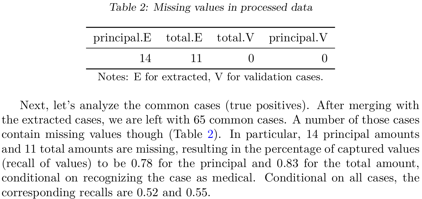
An example research document. This excerpt contains 11 numeric values, all computed from data. If the data is updated, all these numbers must be re-computed and included in the text again.
But what you we want to do both? After all, many reports and other documents contain both titles and bullet lists, but also various numbers and figures that are computed based on data. Obviously, we can compute these numbers in R and just copy over to the document. But in practice, it is hardly ever the case that you can just copy the results to your document. Almost always you must do the computations multiple times as you fix errors, get better ideas and new data. Results in a research paper may have to be updated hundreds of times. Copying all these numbers manually, even once, is a lot of work. Copying those hundreds of times without errors is more than any human can do.
Another thing that neither R nor markdown can do well along is to have access to both code and results. In many cases (e.g. when grading homework 🙂), one wants to see both how certain results are done (the code) but also what are the results. This is hard to do in a code file–you can add the results as code comments, but those are not easy to read, and must be re-written in a similar way like figures in ordinary text. Also, code comments cannot include images.
Rmarkdown offers a solution to both of these problems. You can compute the results using R,7 and write the text about your results using markdown. And both the text and the results will appear in the final rendered version. And when you re-process it, it will automatically redo all the results with no additional manual intervention. Depending on the settings, you may also have the original code visible in the final document, this is a good idea with homework, but probably not a good idea when submitting the quarterly report to your boss. As an additional bonus, you now have your code in the same document (even if not visible in the final version), so one can go and check how exactly did you compute the figures.
The figure below shows an example
rmarkdown document being written (left), and the resulting html in
browser (right). It contains many elements you are already familiar
with, such as text formatting (e.g. **knitting** for bold), inline
code (e.g. `r ncol(iris)`)
and multi-line code blocks
(e.g. the one that begins with ```{r, echo=FALSE}.
Note how in the rendered version at right, the word “knitting” is
bold as in ordinary markdown. But the content of the
code chunks is not printed–instead, the R code there has been
executed and replaced with the
corresponding output. The most striking difference is the plot.
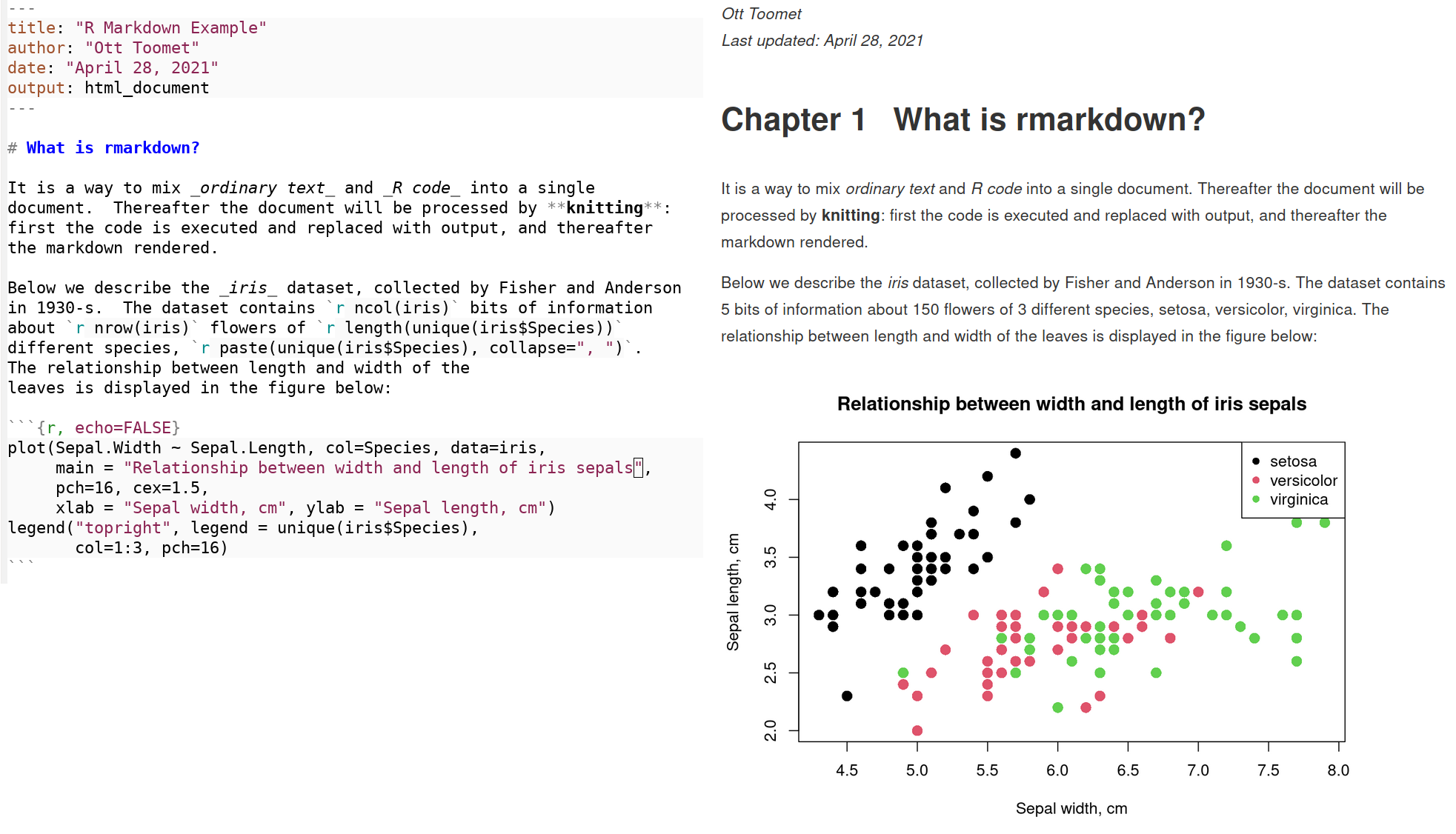
Rmarkdown at work. The left side shows an rmarkdown text being edited with a text editor. Note how the fixed-width fonts, equal line spacing, and also syntax coloring (e.g. string constants are marked red). The right side shows the same document knitted and rendered in a browser: the R code has been replaced by its output, in case of the text paragraph these are the numbers and a list of iris species, in case of the plotting code chunk it is the figure.
Technically, rmarkdown is a markdown document that contains normal markdown text mixed with code chunks, chunks of R code that will run by R like any other R code. Processing rmarkdown takes two steps. The first one is knitting, i.e. running the R code and inserting its output into the document, this converts the rmarkdown document into a plain markdown document. Thereafter one has to render the markdown in a similar way as ordinary markdown. The final result can be html or pdf document, different types of slides, or even MSWord file.
3.5 R Markdown and RStudio
The most convenient way to create and process rmarkdown files is by using RStudio. It includes all the necessary packages and software, and provides easy shortcuts to convert the whole rmarkdown file into the final document with a single click or a keyboard shortcut.
3.5.1 Creating Rmarkdown Files
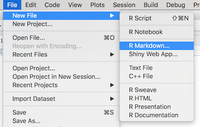
Using the RStudio menu to create a new Rmarkdown document
The easiest way to start a new Rmarkdown document in RStudio is to use the File > New File > R Markdown menu option:
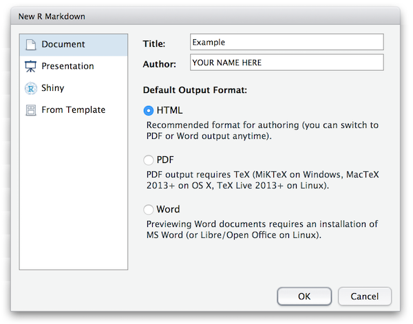
RStudio’s rmarkdown document type dialog
RStudio will then prompt you to provide some additional details about what kind of R Markdown document you want. In particular, you will need to choose a default document type and output format. You can also provide a title and author information which will be included in the document (no worries if you don’t know how to call your document– you can easily change it later). This chapter will focus on creating HTML documents (websites; the default format)—other formats may require additional software.
Note also that working with rmarkdown requires certain add-on packages. RStudio will prompt you to install those–just enable the installation by clicking “Yes”.
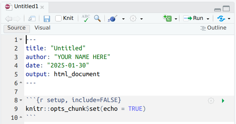
Once you’ve chosen your desired document type and output format,
RStudio will open up a new document file for you. The file contains
some example code (a template) to remind you the basic rmarkdown
syntax. It is a good starting point when you are a beginner, advanced
users may want to just delete the examples.
Rmarkdown files typically have extension .Rmd
3.5.2 Rmarkdown Structure
Unlike plain markdown, rmarkdown files normally begin with header information like
---
title: "My Night at Three Pints Inn"
author: "Ji Gong"
date: "April 28, 2021"
output: html_document
---
This tells R Markdown details about the file and how the file should be processed. For example, the title, author, and date will automatically be added to the top of your document. You can include additional information as well, such as whether there should be a table of contents.
The header is written in YAML
format, which is a way of formatting structured data. But for the
basic headers as what we do in this course, you do not need to know
YAML.
Below the header, you will find three types of content:
Markdown: normal Markdown text like you learned in Section 3.3. For example, you can use two pound symbols (
##) for a second-level heading and asterisks for bullet lists.Code Chunks: These are segments (chunks) of R code that look like normal code block elements (using
```), but with an extra{r}immediately after the opening backticks. The{r}is a crucial marker and tells RStudio that code in these blocks must be executed, not just displayed.RStudio provides a convenient keyboard shortcut,
Ctrl + Alt + I/⌘ + Option + I, for creating new code chunks. See Section J.Inline code chunks: it is also possible to write short code snippets that output a single word or number on the same line as text. For instance, you may write text like
"The answer is`r 1 + 1`". In the final document, this results in a line “The answer is 2”.
3.5.3 Knitting Documents
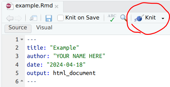
Knit button in RStudio. The corresponding keyboard shortcut is
Ctrl + Shift + K.
RStudio makes it easy to compile your rmarkdown files
into the actual document. This process is called “knitting”.
Simply
click the Knit button (keyboard shortcut Ctrl + Shift + K/⌘ + Shift + K)
at the top of the script panel.
This will generate the document (in the same directory as your .Rmd
file), as well as open up a preview window in RStudio.
Knitting requires certain packages, in particular knitr and rmarkdown (see more in Section 5.6). When knitting for first time, Rstudio helpfully offers you to automatically install the necessary packages. You should just accept this.
If you chose HTML as the output type, RStudio will display the content automatically in a simple built-in browser. If you want to use your “big browser”, you can click the “Open in Browser” button, or just double-click on the html file in your file manager.
3.6 R Markdown Syntax
What makes R Markdown distinct from the plain markdown code is the
ability to actually execute your R code and include the output
directly in the document. R code can be executed and included in
the document in blocks of code, or even inline in the document!
3.6.1 R Code Chunks
Code that is to be executed (rather than simply displayed as code) is
put into code chunk-s. To specify a code chunk, you need to
include {r} immediately after the backticks that start the code
block (the ```). So code chunks should begin with
```{r} instead of the plain markdown code blocks that start with
```.
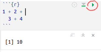
Rmarkdown code chunk in Rstudio.
It begins with ```{r} and ends with
```. The lines between these markers are considered to be R
code and executed. The run button is highlighted in red. Underneath,
its output [1] 10 is visible.
On the figure here is an example
code chunk. Note the beginning marker
```{r} and end marker ```.8
All lines between these
markers are considered to be R code and executed, here it is just
computing the sum 1 + 2 + 3 + 4. The code will normally
be replaced by its output in the final document (but this depends on
the options, see Chunk options
below),
resulting in
[1] 10There are two ways to execute code chunks: you can either knit the
whole document (see Section 3.5.3) or you
can execute them individually. The latter is a very convenient way to
run and develop your code bit-by-bit, and the primary way we do code
throughout this course. You can run a code chunk by clicking the run
button, or use the associated keyboard shortcut Ctrl + Shift + Enter.
Exercise 3.4
Create a new rmarkdown document. Inside a document, write a code chunk that compute the sum of 1 + 2 + 3 + … + 10.- Run the code chunk using the run button
- Run it using the keyboard shortcut
- Knit the whole document.
Are the results similar?
3.6.2 Inline Code
In addition to creating distinct code blocks, you may want to execute R code inline so the result will be part of the text. In this way you can insert individual computed values, such as results you computed in your previous code chunk, directly in your sentences. So if your data or computation change, re-knitting your document will update the values inside the text without any further work needed.
As code chunks are “made” of markdown code blocks, inline code chunks
are “made” of markdown inline code, marked by single backticks
(`). However, you need to put the letter r
immediately after
the first backtick, and follow it with a space and R code, as
`r 3 + 4`. When you knit the text above, the
`r 3 + 4` would be replaced with the number 7.
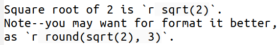
Inline code chunks will result in values right in the text.
The example here shows two inline code chunks. Both are computing root of two, the first one prints it with the default seven digits, the second one rounds it down to only three. Both will be executed and replaced by their output, here 1.4142136 and 1.414. So the final output will look like
Square root of 2 is 1.4142136. Note–you may want for format it better, as 1.414.
In order for the inline code chunks to work, the text must fit on the
single line. So `r 1 + 1` works, but when the
chunk is broken to two lines:
`r, it will just be displayed as ordinary text.
1 + 1`
3.6.3 Chunk execution order
When you knit a document then the following happens:
- Knitting starts with a clean environment, so none of your variables you have defined, or the packages (see Section 5.6) you have loaded are available. You need to define and load those as needed inside the code chunks of your rmarkdown document.
- The working directory (see Section 2.3) of the knitr process will be the folder of your rmarkdown document.
- The code chunks are executed one-after-another, in the order they are written in the document. So if you need a variable defined, you have to write the code to define it above where you are going to need it.9
This workflow may differ from how you normally work with R. It is very common to run the same code chunk over and over again to fix issues, and to execute the cunks back and forth as needed. Unlike knitting, just executing the code chunks has access to R workspace variables and loaded packages. This may result in errors when trying to knit the document afterward, as the code chunks that work in the current environment may not work when started from scratch. It is advisable to knit the document often in order to avoid too many problems when knitting (see Section 3.8.1).
3.7 Chunk options
It is sometimes a good idea to make both code and results visible, e.g. when presenting your coding exercises. However, in other cases either code is undesireable, e.g. when writing the quarterly report to your boss. Or maybe you do not want the results to show up, for instance when doing some kind of auxiliary calculations that you need later but that are not worth of showing to your readers. Rmarkdown offers a large number of chunk options do fine-tune the code execution and displaying behavior. There are two ways to specify chunk options: for a given chunk, and globally.
3.7.1 Chunk-specific options
Chunk options are written in the code chunk header, inside of the
{r} part. They are normally a comma-separated lists of name-value
pairs, e.g. echo = FALSE (this option makes the code invisible in
the final document).
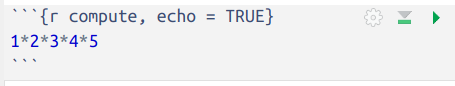
Example of code chunk with name (compute) and a single option (echo=TRUE).
The code chunk example here has a single option (echo=TRUE), i.e. to
show the code in the final document. It also has a name
(compute). The name will be displayed during the knitting
process and it helps in troubleshooting. If you want to set more than
a single option, you need to separate those with commas. For this
code chunk, you might write ```{r compute, echo = TRUE, error = TRUE} to indicate that eventual errors should not break
knitting process but the error message should show up in the final
document instead.
Here is a brief review of the code chunk options. You write code
chunks as ```{r chunk-name, option=value, option=value, ...}
(chunk name is optional).
The first word after
r(and before comma), here chunk-name, is the name for the chunk. Names are good to track knitting, they can also be referred from another chunk, so you can re-use your code chunks. However, an rmarkdown document can only contain a single code chunk with a given name. So you have to change names when copy-pasting your code. If you do not give a name to the chunk, it will be automatically called something like unnamed-chunk-2.echoindicates whether you want the R code to be displayed in the final document (e.g., if you want your readers to be able to see your work and reproduce your calculations and analysis). Value is eitherTRUE(do display; the default) orFALSE(do not display).messageindicates whether you want any messages generated by the code to be displayed. Messages are various startup messages that pop up when you load libraries (see Section 5.6) or files (see Section 12.5.3). Printing (see Section 4.5) is considered output, not messages. This is a good option of you do not want the messages to spoil your final document that should only contain the text and output. Value is eitherTRUE(do display; the default) orFALSE(do not display).includedetermines whether anything – code, output or messages will be included in the final document. The default value isinclude = TRUE, but for certain startup or computing chunks that tend to produce various messages and irrelevant output,include = FALSEmay be a good idea.errorindicates whether you want the knitting to stop and display the error message in case it runs into an error, or if you want it to continue and display the error message in the final document. Values are isTRUE(continue and display the message in the final document) orFALSE(stop, and display the error on the rendering window).For small documents, it is typically easier to display the error message in the final document (
error = TRUE). But sometimes knitr refuses to complete the document at all if there are errors, and then you cannot even see what is the problem unless you send errors to the console (error = FALSE). The latter is also adviseable in case of large documents where you cannot easily check everything for potential errors. It is embarrassing to send your quarterly report to your boss, only for her to discover that it contains big red error messages instead of the expected results!
There are many more options for
creating code chunks. Some of more interesting ones are cache to
speed up knitting and eval for avoiding the code chunk to be
executed.
3.7.2 Global chunk options
RStudio helpfully displays an example of global options as part of rmarkdown template.
The global chunk options are otherwise similar to ordinary chunk
options, but they apply to all following code chunks. But they have
to be specified separately, using knitr::opts_chunk$set() function.
This is normally done at the top of the document in a separate code
chunk.
For instance, if you want to hide all code in your document (but keep
the results visible), then you may write
knitr::opts_chunk$set(echo = FALSE) as displayed on the Figure at
right.
Note that it is in a code chunk with include set to FALSE,
this means nothing from the chunk itself will be visible in the final
document.
For your final report, you may want to hide both code and messages as
knitr::opts_chunk$set(echo = FALSE, message = FALSE),
but if you produce the homework solution, you need to switch the code
back on:
knitr::opts_chunk$set(echo = FALSE, message = FALSE).
3.8 Troubleshooting knitting problems
R-markdown documents are easy to create, and if you write your code correctly, then knitting is just as simple as a keypress. But unfortunately, it is hardly ever the case that one gets the code right in the first try. And code in rmarkdown is harder to debug than just plain R code. There are a few reasons for that.
3.8.1 Knit often
Knit often. Knit each time you have completed a small part of your work, or maybe every 5-10 minutes or so. Use the keyboard shortcut.
This is because you will always make errors. It is much easier to fix the errors immediately, because you know what parts of your document did you change. It may be much harder when you have completed everything–there may be many many problems, and knitting may not even work before you have fixed most of them.
3.8.2 Understand where is markdown, where is code
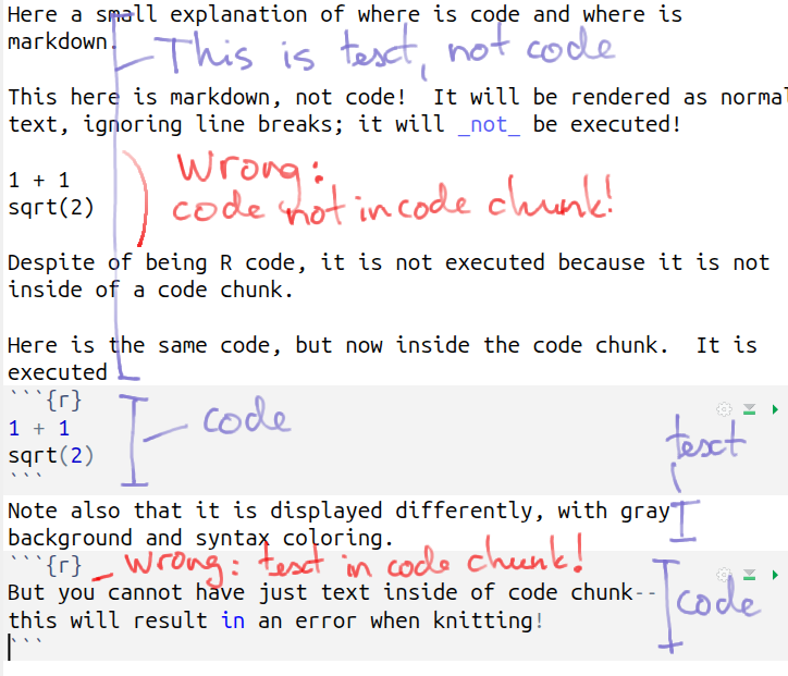
Example of a markdown document where some code is written into plain markdown text, and some text is written into code chunk.
You should understand which parts of your document is code, which parts are just markdown text. Code in plain markdown does nothing and looks like normal text. Code in code chunks will be executed, but any text that is not code will give you syntax errors and may break the knitting process.
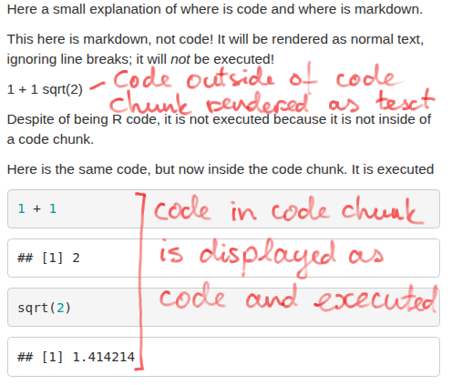
Code outside of code chunk is rendered as normal text.
Code outside of code chunk, just as plain markdown will not be executed. It will not give you any errors, but will be printed on a single line when knitting using normal text font, not the code font.
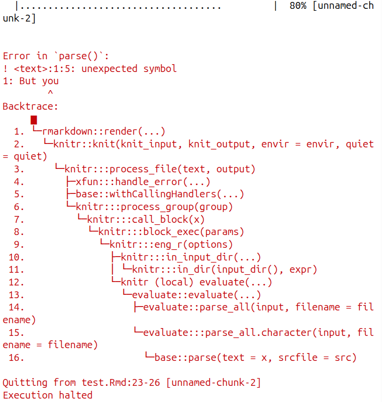
Normal text in a code chunks results in knitting errors.
But if you knit a document where code contains syntax errors,
knitting will fail. Here it happens with the second code chunk,
because it contains normal
text. Knit will throw an “unexpected symbol” error and you will not
even get an html version of your document.
(You may be able to overcome it with error = TRUE chunk
option, see Section 3.7.1.)
3.8.3 Finding errors
Most importantly, the output of your code may not show up neither on screen nor in the document. While you run a plain R script, then the output always appears in the RStudio console. But when knitting, the output may want to your document instead. However, if an error appears then you cannot see output in the document… There are different solutions if you run into this problem:
- Test your code first outside of rmarkdown environment. This is often a good idea, but sometimes it is hard to build a similar environment than the code in your document. For instance, the working directory may be different for knitting and for RStudio console, and hence the file names may not work.
- Use the
error = TRUEchunk option (see Section 3.7 below). This does not break knitting but makes the error message, together with the eventual output visible in the final document. Unfortunately, this does not work with all errors. - Add labels to you code chunks (again, see Section 3.7 below) so you can see in which chunk the problem occurs.
- Remove part of the code from the misbehaving chunk until it works. This may be a slow and tedious process, but it is more general and can be applied to pretty much every coding context.
We also suggest that you write more complex code in a separate script
and then use source() to load script into your document.
This makes it easier to test the more complex data processing outside
of the main document. It also separates data processing from the final
text, this is often considered a good practice.
3.8.4 Knitting is a separate process
A common source of problems is that knitting is a separate process, not the one that that is available as “Console” in RStudio. It is a separate R program that, in particular, has its own working directory. This is the directory where your markdown file is located. It may or may not be the same as the working directory in your Rstudio console!
Knitting is a separate process with a separate working directory!
Besides a potentially different working directory, the knitting
process does not have access to your workspace variables, nor the
packages that you have loaded in console. You need to load data
separately, you need to compute all values in the knitted document,
and you need to load every package with the library() command in
the rmarkdown document. This is to ensure that you can re-compile
your document and get the same result, no matter what other things you
have done in RStudio.
Knitting does not have access to your workspace variables and loaded packages!
3.8.5 Some interactive commands do not work in knitting
Finally, there are commands that do not work when using in
knitting. This includes certain interactive commands
that cannot be included in documents, such as
install.packages(). As it is normally not a good idea to
install packages in documents anyway, we do not discuss the
workarounds.
Use the error message as a useful reminder that one should just load,
not install packages in markdown documents!
Do not use install.packages()
in rmarkdown document!
As a generic advice, you should knit your document frequently and fix the problems immediately before you continue your work. An new error was most likely caused by something you did just a moment ago, and there are good chances that you still remember what did you do. It is harder to fix it later.
3.9 Rendering Data
R Markdown’s code chunks let you perform data analysis directly in your document. It is straightforward with simple numbers, but sometimes you may want to include more complex output in your text. This section discusses a few tips for doing this.
3.9.1 Rendering Strings
If you experiment with knitting R Markdown, you will quickly notice
that print() in a code chunk will generate output that is not very
well suited for a document:
## [1] "Hi there!"For this reason, you may instead generate the message as a string in a previous code block, and display it afterward using an inline chunk (possibly on its own line):
And display it as `r msg`: Hi there!
Note that any Markdown syntax included in the string, such as bold
“Hi” in "**Hi** there") will be rendered as well–the
`r msg`is replaced by the value of the expression
just as if you had typed that Markdown in directly. This allows you to
include dynamic styling if you construct a markdown string out of your
data.
Alternatively, you can also use cat() instead of print() and set
results=“asis”
option which will cause the output to be rendered directly into the
markdown. So
will produce
Hi there!
3.9.2 Rendering bullet lists
Because outputted strings render any markdown they contain, it’s
possible to specify complex Markdown such as lists by constructing
these strings to contain the - or * symbols, and lines separated
by line breaks (either “”, or you can use
multiline strings):
Would output a list that looks like:
- Lions
- Tigers
- Bears
Note: you need to set options echo=FALSE and results=“asis” when printing your output. Otherwise the chunck will render as code chunk, not as markdown.
We can also use paste() (or stringr::str_flatten()) to make such a
list of of a string vector:
predators <- c("Lions", "Tigers", "Bears")
paste("*", predators) %>%  # add '* ' in front of predators
   paste(collapse = "\n") %>%  # combine into a single string with
                           # line breaks in-between
cat() # print- Lions
- Tigers
- Bears
And of course, the contents of the vector (e.g., the text "Lions") could easily have additional Markdown syntax syntax to include bold, italic, or hyperlinked text.
If you do this often, consider creating a “helper function” to do this conversion; or see libraries such as pander which defines a number of such functions.
3.9.3 Rendering Tables
Because data frames are such central features for data analysis,
Rmarkdown includes tools to easily render data frames as
Markdown tables
via the
knitr::kable()
function.10
This function takes as an argument the data frame you wish to render, and it will automatically convert that value into a Markdown table:
| x | y |
|---|---|
| 1 | a |
| 2 | b |
| 3 | c |
kable() supports a number of other arguments that can be used to customize how it outputs a table.
And of course, if the values in the dataframe are strings that contain
Markdown syntax (e.g., bold, italic,
or hyperlinks), they will be rendered as such in the table!
So while you may need to do a little bit of work to manually generate the Markdown syntax, it is perfectly possible to dynamically produce complex documents based on dynamic data sources!
3.10 Homework style guide
This course asks you to do a lot of homework. As common in data science, your tasks are not just coding, but also explaining and interpreting your results. So the result of your homework should not just be good code but a report – a well readable document that contains both code, results, and your interpretation of the latter.
Some of the requirements are generic–whatever you write, you have to ensure that the result is easy to understand for the reader (even if you are just writing for yourself). You have to think about your reader–in the modern world, it is reading time that is the limiting resource. The following requirements are written primarily to make your solutions easily readable for the graders. They also serve as generic suggestions for a “good etiquette” for other tasks, but they may be a bit too specific.
If in doubt, or if you cannot follow the suggestions below, then look at your work with your reader’s eyes. Your reader is your grader. They grader know the questions–you do not have to replicate those here. But can they easily understand your solutions? This is the most important point.
3.10.1 Use rmarkdown and compile your work to html
In this course we use rmarkdown for homework. It is a good way to keep your code and results in one place, and it makes the results easy to read. Unfortunately, it may make it a bit harder to write.
It is critical that you knit your markdown to html. This is what makes it easy for your reader. While markdown text is perfectly human-readable, the reader will not know if your code works correctly. In knitted document it is easily visible. Knit often and fix the issues immediately, see Troubleshooting.
3.10.2 Question numbers
Unlike business reports or research papers, your assignments contain a lot of small questions. And unlike normal papers, they are read by your graders only. But your grader wants to understand which question you are answering. So please:
use 2nd level header (like
## 1.) for the section number (name is not needed)use 3rd level header (like
### 1.1) for the subsection number (name is not needed).use 4rd level headers (like
#### 1.1.1) for question numbers.Students sometimes copy the question itself to the document as well. It is not needed (but it is OK if you do it).
if there are further bullet points, like (a), (b) and so on, you may use just a bullet list for those, and mark the bullets (see the example). Sometimes, if all questions are about coding, you can add (a), (b), and (c) in code comments instead. Other times is clear enough, so you may skip the letters altogether. In any case, ensure that it is clear enough which subquestion you are answering.
See the example below.
3.10.3 Code and text
Rmarkdown is good for both code and text if used correctly.
- use normal text (normal paragraph) for explanations. Use different
fonts, such as bold and italic as appropriate. Do not use code
comments, and
cat()orprint()statements for text explanations! - no explanations are needed for simple code questions that result in a single number or text, something that your reader can immediately understand.
- use R code chunks (
```{r} ... ```) for code. - keep code visible (
echo = TRUE, see Chunk options). If your code spits out a lot of irrelevant messages (e.g. when loading tidyverse library), consider making messages invisible (message = FALSE). - Keep your code lines of suitable length–all your code should be visible on normal screens. 80-90 characters is typically a good choice.
- Use code comments (
# ...) as appropriate to explain your code. Do not use it to explain the results. In general, you should comment more complex code parts, trivial parts should not be commented. - Your code should normally produce output–your calculation
results should be visible. However
- not all code makes calculations. E.g. if you are asked “create variable my_age that equals your age”, then there is no reason to show any output.
- not all output is worth showing. For instance, if asked to “load data, and keep only persons born in 2003”, then we do not want to see potentially thousands of lines of data.
- do not print out a lot of data, or produce otherwise excessive output. It is all right to show a few lines of data, or to print max and min values, or a summary table. It is not OK to print thousands of lines of data.
3.10.4 Example
Here is a very simple example.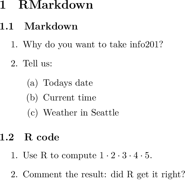
At right is the pdf text of an example problem set. It contains a single section (“1 RMarkdown”) and two subsections (“1.1 Markdown” and “1.2 R code”). It contains multiple questions, e.g. “1. Why do you want to take info201?”. This question can be referred to as 1.1.1. Question 1.1.2 contains three subquestions ((a), (b), (c)).
Subsection 1.2 are just text questions and should be answered in markdown. 1.2.1 is a coding question that does not need any comment by itself. You should answer this as computer code in a code chunk. But if needed, you can add comments and explanations, either as code comments or markdown text, as appropriate. 1.2.2 asks you to comment the previous result. This is, again, a text question, so you should answer this in markdown.
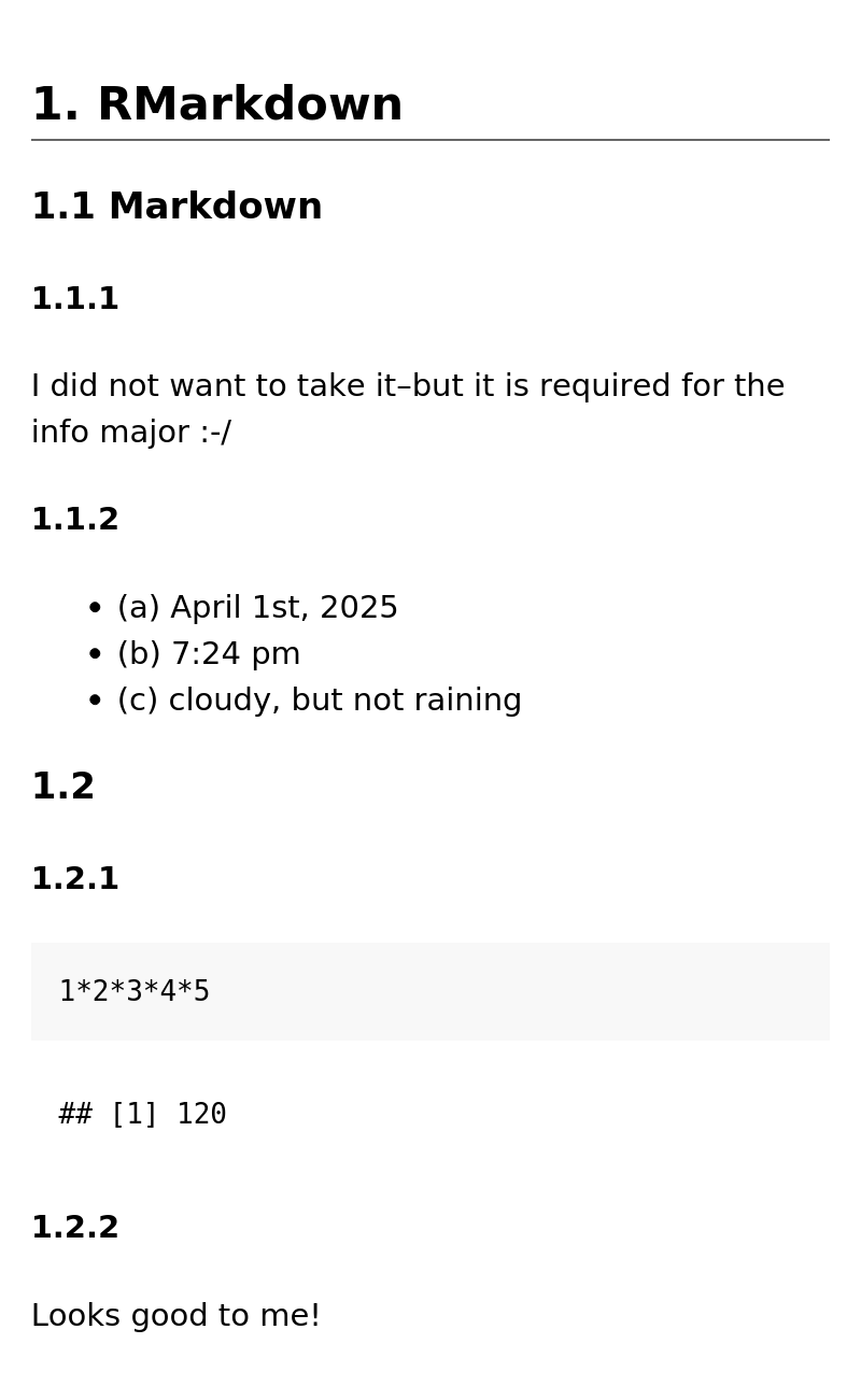
## 1. RMarkdown

### 1.1 Markdown

#### 1.1.1

I did not want to take it--but
it is required for the info major :-/

#### 1.1.2

* (a) April 1st, 2025
* (b) 7:24 pm
* (c) cloudy, but not raining

### 1.2

#### 1.2.1

```{r}
1*2*3*4*5
```

#### 1.2.2

Looks good to me!
It is formatted along the specifications above:
- sections as 2nd level heading
## - subsections as 3rd level headings
### - questions as 4th level headings
####. The example includes the long question numbers like#### 1.1.1and#### 1.1.2, but if it is clear enough, then just#### 1and#### 2may be enough. - the subquestions are formatted as a bullet list with
(a),(b)and so on. Here it works well. - R code is in a code chunk. The result (
[1] 120) is clearly visible, no further explanations needed. - 1.2.2 contains your comment, written as markdown text.
TBD: figures for homework style guide
3.11 R Notebooks
An alternative (or more like a complement) to rmarkdown is to use “R Notebooks”. R Notebooks are very similar to rmarkdown–actually there is no difference in the files itself, just the way how the code chunks are run.
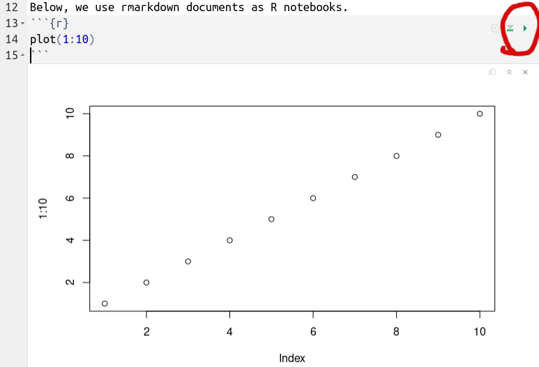
Example of a rmarkdown code chunk. It can be run using the circled
green triangle button at right, or by pressing Ctrl-Enter. This
makes the chunk to run, its output will be displayed underneath.
Note that the code chunks have three special buttons at the top-right corner. The green arrow (circled on the image) makes the chunk to be run as a “notebook cell”. This means the chunk is run, and its output is displayed underneath of it–in this figure this is the plot. This is a very handy way to run the individual code chunks, test and debug them, and see what is the output.
But when using rmarkdown documents as notebooks, be aware of the following caveats:
- Notebook chunks are run in the current R instance, the R program
that is running in Console at bottom right pane. Hence the
chunk’s working directory is the same as the current R instance’s
(the one you can check with
getwd()), and it has access to all your workspace variables and data. This may cause problems when you rely on these things–remember, the knitting process is run in a separate R instance that may have a different working directory and that does not have access to workspace variables. - Rmarkdown documents only work as notebooks inside of RStudio. If, for some reason, you do not use RStudio, then you cannot run it as a notebook. You can still knit though–it just requires a few commands that you do not have to memorize when using RStudio.
If you are running your code as notebooks, it is still advisable to knit your document frequently, in order to avoid too many compilation issues later.
The program is called pandoc, and it is automatically installed when you install RStudio.↩︎
In case of more complex tables, you can use helper tools, such as online table generators. Just search for one!↩︎
You can also use other languages, such as python↩︎
We strongly recommend to use the keyboard shortcut
Ctrl + Alt + I/⌘ + Option + I, to create code chunks. This saves you a lot of time. See Section J.↩︎It is also possible for one code chunk to call another one. See knitr documentation for details.↩︎
knitr::kable()is a way to refer to the functionkable()that lives in knitr package. It is equivalent (mostly) to loading the knitr library withlibrary(knitr)and then using justkable().↩︎