Chapter 4 Introduction to R

R logo. © 2016 The R Foundation (CC-BY-SA 4.0).
R is a powerful programming language and environment for data analysis. It is one of the most popular data science tools because it is designed from ground up for statistics and data analysis. It is the programming language used throughout this book.
This chapter is primarily designed for readers who have little to no experience with programming, and hence we devote quite a bit of space to topics like variables and data types. If you have programming experience, you may quickly skim through this chapter to just learn the basic R syntax, and how to use RStudio.
4.1 What is R and why do you want to use it?
R is a programming language that allows you to write code to work with data. It is designed from ground-up for this task–statistics and data processing.
R is called “R” because it was inspired by and comes after the language “S”, a language for Statistics developed by AT&T.
There are many other languages that are good for working with data. We have selected R because of its simplicity–as a language that is designed for such tasks from ground up, its tools are rather simple. This is also a reason why R is very popular in areas like health and social sciences–data processing in R is typically easier and requires less coding than in more general languages.
Working with R (and other programming languages) works by writing formal instructions to your computer, and the computer will execute those. The instructions can be written in different “languages”, more precisely programming languages, and the computer needs tools to understand each of these. R software you installed above (see Section 1.1) is one such tool.
As projects grow, it will become useful not to issue the instructions one-by-one, but to write them all down in a single file, and then tell the computer to execute all of those instructions. This list of instructions is called a script or program or code. Writing scripts is called programming or coding. Executing or “running” a script will cause each instruction (line of code) to be run in order, one after the other, just as if you had typed them in one by one. Writing scripts allows you to save, share, and re-use your work. By saving instructions in a file (or set of files), you can easily check, change, and re-execute the list of instructions as you figure out how to use data to answer questions.
As you begin working with data in R, you will be writing multiple
instructions (lines of code) and saving them in files with the
.R extension, representing R scripts.
Through this course we use RStudio for this task, but if you wish, you
can use any text editor.
4.2 Basic R
Here we introduce the very basics of R language. We start with typing simple commands on console, and thereafter switch to scripts or rmarkdown. If your task requires just 1-2 commands, then it is often easier to type those directly on the console (the lower-left pane in RStudio). But if you need more than just a few commands, then it is usually easier to use rmarkdown (see Section 3.6) or scripts (see Section 4.2.2 below).
4.2.1 Entering commands on console
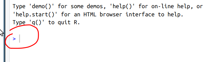
R prompt in the R console window, followed by command 1 + 1.
R Console is a small window where you can type in R commands.11
It is normally the lower-left pane in RStudio.
The commands must be typed after the R prompt >. The prompt
is a marker that R is ready and is waiting your commands.
We can start with simple arithmetic. Write
1 + 1 in the R command prompt and hit enter.
R replies with [1] 2. Below we write these steps as:
## [1] 2The first block shows the commands you issue in R console, and
underneath
is ## followed by the R’s reply (the answer). The R’s reply
contains the answer, 2, and a marker [1]. The marker is related
that to the fact that
one command may produce many answers and this is the first of those
(see more in Section 6 below).
The normal R prompt is >. However, sometimes R expects you to
continue the previous command, in that case the prompt changes to
+. You can get the normal prompt back with Esc. See Section
4.2.2 below.
This is how we can use R as a powerful calculator. The other
arithmetic operations are pretty easy and intuitive: - for
subtraction, * for multiplication, / for division and ^ for
exponentiation. Only exponentiation is somewhat non-standard,
different programming languages have different habits here. R knows
that multiplication must be done before addition, if you want the
opposite then you need parenthesis:
## [1] 7## [1] 9Let’s now compute something that is hard to do manually–namely the length of light-year. Light-year is the distance that light, moving 300,000 kilometers per second, covers in one year:
## [1] 9.4608e+12Here we take the speed of light, and multiply it by seconds in minute (60), minutes in hour (60), hours in day (24) and days in year (365). R prints the answer in exponential form, it must be understood as \(9.46\cdot 10^{12}\), i.e. almost 10 trillion kilometers.
You cannot just click on the previously entered command and edit it. But in RStudio, you can use the up arrow to retrieve the previously entered command, edit it, and re-run.
See more in Section J.
R Console understands R commands but it does not understand markdown. Markdown commands, when entered in R console, will either do nothing, or cause an error.
4.2.2 Writing scripts
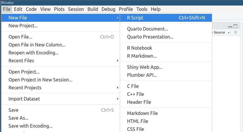
One can open a new script through RStudio menus, the corresponding keyboard shortcut is visible as well.
Section 3.6.1 above discusses how to include R code in rmarkdown documents. This is a good idea if you want to have both text and computing results in a document. But it is not a good solution for all tasks. For instance, sometimes you only want the results printed on screen. Or you want your computer to control a website instead. In those cases the best solution will be a script. Scripts are basically just lines of R code, written underneath each other. Or if you want–a script is a giant code chunk without any markdown.
The easiest way
to write scripts is by using the RStudio script editor. Depending on
your exact configuration, an “Untitled” script may already be open, or
you can choose from menu File
-> New File -> R Script (or Ctrl - Shift - N).
This opens a new R script in a dedicated
window (top left in RStudio).
Let’s put the same R command in that window. Now the command (or more often, a collection of commands) is called script or computer program.12 So the content of your script window will look like
This is a script, a very simple, one-line computer program.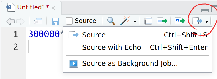
Location of “Source” button in R Script window in RStudio.
The next task is to run the script, it means execute all the commands there (or in this case the only command we have there). RStudio offer several ways to do it:
- “Source” (Ctrl + Shift + S) will execute (source in R parlance) the program. It will not show the code that you execute, nor any results that are not explicitly printed (see Section 4.5).
- “Source with Echo” (Ctrl + Shift + Enter) will also execute the code, but will show both the code and output, even if not explicitly printed.
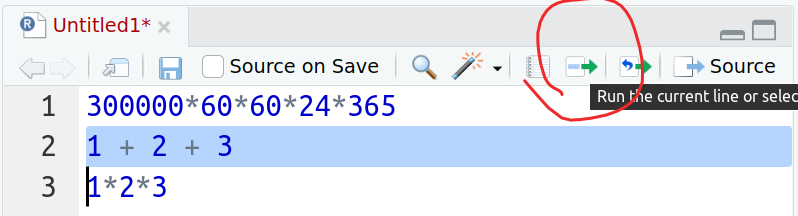
Location of “Run” button in R Script window in RStudio.
Another handy way to execute code is to use “Run” button (Ctrl + Enter / ⌘ + Shift + Enter). This executes either the region that is highlighted, or the command where the cursor is currently located if there is no highlight. In the example figure at right, this will execute the line “1 + 2 + 3”, and show both the code and the result in the “Console” window.
Finally, you may want to save your script using a better name than “Unititled”. Use the menu: File -> Save As… to pick a good name.
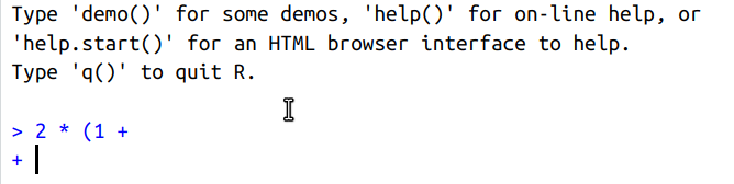
If R thinks that you are not ready with the command, it shows +
instead of >.
Sometimes it happens that you either write your script wrong, or you
run only a part of it. In that case you may notice that the normal
command prompt > is replaced by continuation prompt +. This
is because R thinks that you are not ready with the command and
expects you to continue.
The image here demonstrates how this can
happen. After entering 2 * (1 +, R does not see the closing
parenthesis and concludes that you will continue the command. You may
notice that “nothing works” until R has understood that the command is
finished. Here you can just enter the closing parenthesis ), but
otherwise the Esc key will help. Pressing Esc will interrupt the
incomplete command and restore the normal command prompt.
4.2.3 Comments
One of the extremely handy and simple features of computer code are comments. These are part of the code that are ignored by computer. These are just notes for the human reader (including you!) to make it easier to understand what the code does. Since programs can be opaque and difficult to understand, comments are widely used to add explanations. Even your own code may be incomprehensible to you only a few weeks after you wrote it.
Comments should be clear, concise, and helpful—they should provide information that is not otherwise present or “obvious” in the code itself.
In R, we mark text as a comment by putting it after the pound/hashtag
symbol (#). Everything from the # until the end of the line is
a comment. It is common to put descriptive comments immediately above
the code it describes, and sometimes immediately aftewards. One can also put short notes at the end of the line of code:
So the commented light-year code might look like this:
## Length of light-year:
## c by seconds in minute by minutes in hour by
## .. by hours in day by days in year
300000*60*60*24*365
Note that these comments start with double hash sign ##: only one is
needed, but as the computer ignores everything after the first one, it
will also ignore the second one. So any number of hash signs is fine!
See Section 9.5.2 for more about how to write good comments.
You can “execute” comments and enter those on the console, but it is not very useful as they do not do anything.
Comments are also used for temporarily “deleting” parts of the
code–if you add comment signs # in front of every line in some
parts of your code, these lines will be ignored by the computer (it is
called “commented out”). But
you can easily get these back if you need those again.
In RStudio, you can turn highlighted lines into comments and back to
code by
pressing Ctrl - Shift - C. See more in Section
J.
4.3 Variables
Since computer programs involve working with lots of data, we need a way to store and refer to this information. We do this using variables.
4.3.1 What are variables
For instance, if you want to add numbers, we can do just write it as
## [1] 7This is a good way to compute something where we know the inputs
(numbers “2” and “7”) and we just want to see the output. But quite
often we want to do something similar, just we do not know what are
the numbers. It may sound a bit counter-intuitive–how on earth can
you compute something if you not know the inputs?
But there are many valid
reasons for that. For instance, we may ask the input from the user. Or
the input may be date or time, and we do not know when will someone
run our program. Or the input is read from a dataset, and it may be
one of many datasets. In such cases can we cannot “hardcode” our
computations like 2 + 7. We must keep the program open to learn the
actual input values later. This can be done using variables.
The same example above, just using variables, may look like13
## [1] 7So what is the difference? After all, we still got the same number?
However, now our code stores the numbers, “2” and “7”, in memory under
two separate labels (variable names) “x” and “y”.
You can think of variabls as labeled “boxes” for data. You can
use the label to refer to the data inside. The numbers can be stored
into the boxes (variables) using a
special assignment operator <-, it is like an arrow that puts
number
“2”
into a box labelled “x” and number “5” into the box “y”. This process
is called assignment. Note that variable names goes left, value
comes right.14
Later, we just
use the box labels (variable names) to perform the tasks with data
that is
inside of the boxes (variables).
In RStudio, use Alt-- (Alt-minus) to get the <- operator.
See Section J for more.
Now you can imagine that instead of x <- 2 and y <- 5, we may
instead write code that asks x from the user, and reads y from a
dataset. But computation, adding x and y, will remain
the same. This is the beauty of
variables: as long as the computations are the same, we can use the
same code.15
But variables can also be used to remember and retrieve the values later. This requires a slightly different code, for instance:
## [1] 7Note that we store the result of x + y in “z” in a fairly
similar manner as how we stored numbers into “x” and “y”. Just what
goes into the box “z” is a result of a calculation, not a given number
as above.
Now we have an
additional “box” in memory, labeled as “z”. You can see your variables in
RStudio “Environment” pane. You can also see all the variables using
command ls():
## [1] "x" "y" "z"This shows that we have defined three variables: “x”, “y” and “z”.
More specifically, we are talking here about workspace variables or environment variables. These are the variables that are part of R workspace, and that you can see on the top-right “Environment” tab in RStudio. These are what programming languages typically call just variables. Later, in Section 12, we will encounter data variables, stored in the datasets instead of the workspace.
A note about the last line–it is just “z” and nothing else. This is for printing the result. Rmarkdown normally only prints the result if it is not assigned to a variable. If we were writing the code instead like
then we do not see any result. The result is still computed, just not printed on screen. The last lonely “z” prints it in a simple manner (see Section 4.5 for more about printing).
We can use any variable to do computations and store it in any variable. So we can also do like this:
## to begin with, 'z' contains value '7'
z <- z + 1  # take z, add 1, and store result back in z
z  # now it is '8'
## [1] 8Here we take the number form the “box z”, add “1” to it, and “put it back into the same box”. This is perfectly valid computer code, and in fact widely used for various tasks, such as counting.
4.3.2 Variable names
In the example above, we used a single-letter variable names. But
they need not to be single-letter only, they may be much longer. In
fact, you are fairly free to choose any kind of names you want but
there some rules:
variable names must begin with a letter and can contain any
combination of letters, numbers, periods (.), or underscores
(_).
Here are a few examples of valid variable names:
All these styles have their advantages and disadvantages, in general, pick shorter names for shorter scripts and long descriptive names for large complex projects. You can pick all kinds of variables names, but they should be descriptive and informative about what the “boxes” contain. Confusing or misleading variable names is a major problem in programming. See more in Section 9.5.1.
A good example of how to use variables and choose variable names is here:
Variable names are case-sensitive, so “x” and “X” are two different
variables. In the example above, Minutes_in_day will not work:
## Error in eval(expr, envir, enclos): object 'Minutes_in_day' not foundHere are some examples of invalid variable names:
This code will not work and produce errors.
Exercise 4.1 When coding, it is important to understand the error messages. Type these invalid assignments in RStudio console. What are the exact error messages you get?
See the solution
Variable names must begin with a letter, but it does not have to be English letter. Any UTF-8 letter is fine. So you can write code like
## [1] 5You can see what value is inside any variable by typing that variable name as a line of code:
## [1] 14.4 Data Types
In the previous section, we were only working with numeric values. We did some computations and stored those in variables. But there are data that are not numbers.
The two most important non-numeric data types are text (strings) and logical values. Using other data types is very similar to using numbers. For instance,
R is intelligent enough to understand that if we have code x <- 7,
then x will contain a numeric value (and so we can do math with
it!), and if your write y <- "blah-blah-blah", then it is text, and
we can convert it to upper case instead.16
There are four “basic types” (called atomic data types) in R that we encounter in this book.
4.4.1 Numeric
The default computational data type in R is numeric
data. It can represent real numbers (numbers that
contain
decimals). We can use use mathematical operators
(such as +, -, *, ^, see below in
Section 4.4.1)
to do computations with numeric data. There are also numerous
functions that work on numeric data (such as calculating sums,
averages and square roots).
Numeric data is normally printed in a fairly obvious way, e.g.
## [1] 0.5In case of non-finite fraction, only the first few digits are printed:
## [1] -0.1428571If numbers are too large, or too small, then they are printed in exponential form:
## [1] 2.181818e+13## [1] 1.666667e-10The exponential form must be understood as \(2.181818\cdot10^{13}\) in the first case, and as \(1.666667\cdot 10^{-10}\) in the second case. Exponential form can also be used to enter numbers, e.g.
## [1] -0.03Naturally, there are various ways to adjust the way the numbers are printed.
There is also a special mathematical constants: pi is
\(\pi = 3.1415927\), and Inf is infinity.
You can get infinities when you do certain operations, e.g. divide
by zero. You can also use infinity if you need a constant that is
larger than any number.
One can use Mathematical operators with numeric values.
Mathematical operators are the common signs like + and - that
allow to do basic mathematics (to “operate”), plus a few others:
+: addition-: subtraction*: multiplication/: division^: exponentiation (i.e.2^3means2*2*2).
These are defined for most numbers, except for a few corner cases, such as division by zero. The other way to do math, besides operators, is with functions. We’ll talk more about those below in Section 5.2.
Besides these well known mathematical operations, there are more, for instance
%/%is integer division: e.g.7 %/% 2equals 3. This is a division that only returns the integer part and ignores the remainder.%%is modulo, e.g.7 %% 2equals 1–when you divide 7 by 2 you get 3, and 1 is “left over”.
There are many more mathematical operators, such as matrix product or outer product. We do not discuss these in this book.
Exercise 4.2 Use integer division to transform years to decades. E.g. 1966 → 1960 and 2023 → 2020.
See the solution
4.4.2 Character
Another very common task we do is to perform simple text manipulations. Text data is called character or string data in R. This may include simple tasks like storing a single letter in a variable, or changing words to upper case; but it may also include quite complicated text analysis.
You can tell that something is character data by putting this in
quotes (both single quotes ' and double quotes " will do).
For instance, we can store the name of a certain well-known playwriter
in a variable:
Note that character data is still data, so it can be assigned to a variable just like numeric data! We can print its value by just typing its name on the console, or using dedicated printing functions (see Section 4.5). There are no special operators for character data, though there are a many functions for working with strings.
Note that it is not the content but the type of the content that decides if the variable is numeric or character:
Both variables contain “one”, but in case of “x” this is stored as
number, in “y” it is stored as string. This is because 1 (without
quotes) is a number and "1" (with quotes) is a character, and the
variable automatically “knows” what type data you put in there.
Hence we can do mathematical
operations with “x” but not with “y”, and text functions with “y”
but not with “x”:
## [1] 2will work but y + 1 will give an error. If you are unsure what
type of a particular variable is, you can query it with function
class(), e.g.
## [1] "character"Exercise 4.3 Try to add a number to y. What is the exact error message? Do you
understand what it tells?
There are no dedicated character operators but there is a plethora of functions that can manipulate text.
Only standard double quotes ("") and standard single quotes ('')
can be used to create strings. Various kinds of “fancy quotes” will
not work. If you try to do this, you’ll get an error:
## Error: <text>:1:6: unexpected invalid token
## 1: s <- “
##          ^
As the quotes are rather similar, this may create hard-to-spot problems.
However, you can use fancy quotes inside strings as any other character:
See Section 21.1 for more details about character strings.
4.4.3 Logical
The third extremely important variable type is
logical variables (a.k.a Boolean variables). These can only store
two values–“true” or “false”.
In R, these two values are written as TRUE and
FALSE. Importantly, these are not the strings "TRUE" or
"FALSE"; logical values are a different type! If you write
these values as code in RStudio,
you see that it has a special color for these “logical constants”.
logical values are called “booleans” after mathematician and logician George Boole.
But why do we need such “powerless” variables that can only contain two values? Weren’t it more useful to use numbers or strings that can do much-much more? It turns out that logical values are extremely important. Namely, most of decision-making is logical. We either do this, or we do not do this. And there is a lot of decision-making in the computer code. We have to check if our results are correct or not, if the user input makes sense or not, if we are done with all inputs or not, so forth. All these decisions involve only two values, and R has many decisionmaking tools that rely on such logical values (see Section 10).
You can create logical variables directly, like a <- TRUE but that
is rarely useful. Most commonly we see those as
the result of applying comparison operators to data.
These are
<: less than>: greater than<=: less-than-or-equal>=: greater-than-or-equal==: equal!=: not-equal
Note that equality is tested with double equal signs ==, not with
single equal sign! For instance
## [1] FALSEgives you FALSE but you cannot use single equal sign for comparison,
2 = 3
gives an error instead.
Comparison operators behave in many ways exactly as mathematical
operators like + and *, just they result in logical values:
## [1] TRUE## [1] FALSEWe can store these values in variables exactly like in case of numbers or strings:
## [1] FALSEHere are a few more examples
## Is the product cheap?
price <- 20
cheap <- price <= 10  # if price no more than 10, we call it 'cheap'
cheap  # FALSE: it is not cheap
## [1] FALSE## Do these screens have equal number of pixels?
screen1 <- 3840*2160 # 4k widescreen
screen2 <- 5120*1440 # 1440p ultrawide
screen1 != screen2 # do they have different number of pixels?## [1] TRUE## [1] TRUENote how in case of screens, we left if to R to compute the actual number of pixels–we do not have to compute it ourselves. The computer can do it for us.
Exercise 4.4 Are you more than 20 years old? Assign you age into a variable,
compare this to 20, and store the result in another variable. Finally
print it, it should print TRUE or FALSE, depending if you are
older than 20 or not.
See the solution
One can also compare strings. While equality is fairly obvious, then for instance
## [1] FALSEturns out to be false. This has nothing to do with the size of the corresponding mammals–the fact that cat is “smaller” here means it is located before dog when written in alphabetic order.
See more in Section 7.2.
Logical values have also additional operators, called logical operators or boolean operators. These work only with logical values and they produce logical values. This allows you to make more complex logical expressions. Although their behavior is very similar to that of mathematical operators, logical operators are often confusing for beginners. We are used to work with numbers but not with logical values.
Logical operators include &
(logical and), | (logical or), and ! (logical not). The meaning
of these logical operators corresponds rather closely (but not
exactly!)
to their meaning
in everyday language. In particular true AND true is true, for
instance
## [1] TRUE## [1] TRUE## [1] TRUEBut if any of the involved logical values is false, then logical AND will produce false:
## [1] FALSEHowever, you can use logical NOT, ! to reverse the condition:
## [1] TRUENote that we need to put x > 4 in parenthesis to tell R that !
applies to x > 4, not on x alone!
Logical OR behaves otherwise similarly, but it is true if at least one of the values involved is true:
## [1] TRUE## [1] TRUEIt’s easy to write complex expressions with logical operators. If you find yourself getting lost, I recommend rethinking your question to see if there is a simpler way to express it!
Exercise 4.5 Use the pet example above to deduce if you are happy and it is raining today. You may write it in a way as
Your code should print TRUE or FALSE depending your mood and
weather.
See the solution
4.4.4 Integer
The final “atomic” data type we encounter in this book is integer. These are numbers like “numeric”, but these can only hold integer values. Now again, one may ask why do we need such limited numbers, but there are a few reasons for this.
- First, and most importantly, integer arithmetic is precise. This is not guaranteed to be the case of floating point “numerics”–computers cannot represent infinite number of decimals, and hence usually only produce results that are close to, but not exactly right.
- The other reason why integers is sometime preferred is that integer arithmetic may be faster and consume less memory. However, for computations we encounter in this class, the storage and computation speed does not matter.
Integers are produced by certain operations, e.g when creating sequences.
Base R has two additional “basic types” that we do not discuss in this book:
- Complex: Complex (imaginary) numbers have their own data storage
type in R, they are are created using the
isyntax:c <- 1 + 2i. - Raw: is a sequence of “raw” data. It is good for storing a “raw” sequence of bytes, such as image data. R does not interpret raw data in any particular way.
4.5 Producing output: cat and print
When you just compute on R console, knit a code chunk
or even when you write small
scripts, it is not necessary to dedicate any extra effort to printing. The
results are automatically printed. This is a common behavior in R
console: the last result will be printed. It is a handy but limited
feature.
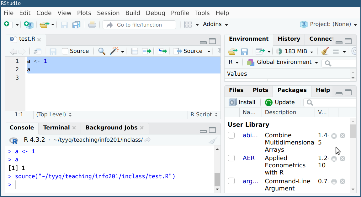
Output depends on the way the code is executed. The same script is
first “run”, that produces the first lines of output on the console,
including the result “1”. Thereafter it is “sourced”. The only
prints the source() command, but no output.
First, it only prints the “last” value (unless assigned to a variable). Second, this only works in certain environments, e.g. in RStudio console when running the program, but not when “sourcing” it (see Section 4.2.2). Third, when writing longer programs, you may want to see more results than the last one, and maybe also add some explanatory notes. Finally, the result depends on what exactly does the “last” value mean–the code can either be fed line-by-line, in which case every value is the last one, or all at once, in which case only the last line is the last one…
All this suggests that instead on relying automatic printing, in more
complex projects you may want to use dedicated printing functions.
R has two printing commands: cat and print. cat is useful
if you want to print simple objects, but potentially more than one
object. These may be one or more numbers, strings, and
explanatory text. print can output complex objects but only one at
time.
Next, we illustrate the usage of cat:
## Compute length of light-year
ly <- 300000*60*60*24*365
cat("Length of light-year is", ly, "km\n")
## Length of light-year is 9.4608e+12 kmThis code chunk computes the length of light-year and prints it with a small informative message. Alternatively, we can just compute this number and let R console to automatically print it:
## [1] 9.4608e+12Why should we use cat then? The automatic printing is good enough
if you work interactively on console, or just run very short code
snippets. But if the code is not run on R console, then
the number may not
even be printed. Alternatively, if the script computes and prints
many results, the user gets easily confused what do these numbers
mean. So it is a good habit to output your results together with a
brief explanation.
The syntax of cat is pretty simple: it takes a list of arguments,
texts, variables and numbers you want to print. One very useful
symbol you may want to add is the
newline character "\n". (Note: it uses backslash "\n", not
_slash "/n".) This forces
printing to jump to the next line:
## hi there## hi
## thereprint is somewhat similar to cat but designed to output more
complex objects, such as vectors, lists, and
data frames. Print may produce multi-line output but
it does not allow to add explanatory messages. You have to cat the
message and print your complex object thereafter.
Obviously, output does not have to be printed on console, it may also be sent to a file, or uploaded to internet, or played as audio instead. But whatever the exact format, it is important to ensure the user has enough information to understand what the output is.
Finally, let’s use the tools we learned above, and re-write the light-year script in a way that looks more like normal computer code:
## Compute the length of lightyear
c <- 300000  # speed of light (km/s)
lightMinute <- c*60
lightHour <- lightMinute*60
lightDay <- lightHour*24
lightYear <- lightDay*365
cat("Lightyear is", lightYear, "km\n")
## Lightyear is 9.4608e+12 kmExercise 4.6 How long it takes for sound to travel around Earth?
- Speed of sound is 0.34 km/s
- Circumference of earth is 42,000 km
- Write a similar script that computes the time in seconds, hours, and days.
- It should print something like Sound travels around Earth in xxx seconds or in yyy hours, or zzz days
See the solution
4.6 Getting Help
Humans make errors. It is impossible to write anything resembling a substantial computer program without dozens of errors in the process. Programmers spend a considerable amount of time trying to find and correct errors (this is called debugging). Here are a few suggestions about how to get help.
Read the error messages: If there is an issue with the way you have written or executed your code, R will often print out a red error message in your console. Do your best to understand the message–read it carefully, and think about what is meant by each word in the message. You may also put it directly into Google and see if you can get better explanations. You’ll soon get the hang of interpreting these messages if you put the time into trying to understand them.
Google: When you’re trying to figure out how to do something, it should be no surprise that Google is often the best resource. Try searching for queries like
"how to <DO THING> in R". More frequently than not, your question will lead you to a Q/A forum called StackOverflow (see below), which is a great place to find potential answers.StackOverflow: StackOverflow is an amazing Q/A forum for asking/answering programming questions. Indeed, most basic questions have already been asked/answered here. However, don’t hesitate to post your own questions to StackOverflow. Familiarize yourself with how to ask questions on StackOverflow though.
It happens often that by the time I can articulate the question clearly enough to post it, I’ve figured out my problem anyway.Documentation: R’s documentation is actually quite good. Functions and behaviors are all described in the same format, and often contain helpful examples. To search the documentation within R (or in RStudio), simply type
?followed by the function name you’re using (more on functions coming soon). You can also search the documentation by typing two questions marks (??SEARCH).You can also look up help by using the
help()function (e.g.,help(print)will look up information on theprint()function, just like?printdoes). There is also anexample()function you can call to see examples of a function in action (e.g.,example(print)).rdocumentation.org has a lovely searchable and readable interface to the R documentation.
chatGPT and similar AI applications can generate code for you, if you know what to ask. It may not be correct code, and it may not be exactly what do you want, but it is advisable to familiarize yourself with such tools. It is not a substitute for basic manual coding though–it is important you know the basic programming tools and syntax, among other things it also helps to evaluate the suitability of AI-offered solutions.
See Section 9 for more information about learning, getting help, and debugging.
4.7 Summary
R prompt: marker “
>” in R Console, marking that R is ready to accept your commands. See Section 4.2.1.Sometimes it turns into continuation prompt “
+” that does not accept commands, pressEscto get back to “>”. See Section 4.2.2.Script: a number of commands written underneath each other, to be executed sequentially. In RStudio, highlight the lines and press Ctrl + Enter, or Ctrl + Shift + S. See Section 4.2.2.
Variables: labeled location (“boxes”) in memory that contain values. Variable names must begin with a letter, and can contain letters, numbers, underscores
_and dots. Variable names can be used instead of the corresponding values. See Section 4.3.Data types: computer stores data in 3 different ways:
- numbers:
a <- 3 - character:
b <- "hi there!"(must be in quoted) - logical:
c <- TRUE
See Section 4.4.
- numbers:
Producing output:
- use
cat()to print multiple items with explanatory text:
cat("I am", age, "years old and I live in", city, "\n")
- use
print()to print single item, on multiple lines if needed, such as a dataset.
See Section 4.5
- use
Help: using
?function_name
brings up the help page forfunction_name(). Use
??topic
to find the help pages, relevant for the topic. See Section 4.6.
Resources
- R Tutorial: Operators
- R Documentation searchable online documentation
- R for Data Science online textbook, oriented toward R usage in data processing and visualization
- aRrgh: a newcomer’s (angry) guide to R opinionated but clear introduction
RStudio also contains a system command shell, labeled “Terminal”. Do not mistake it for R console, labeled “Console”. It will not understand R commands.↩︎
There is no clear distinction between script and program. Typically, one calls simple programs “scripts” and more complex programs “programs”. Also, programs written in compiled languages are rarely called “scripts”. So writing scripts is “programming”.↩︎
Those who are familiar with statically-typed languages, such as java or C++, may notice that we do not have to declare the variables nor their types. R will figure it out automatically. One can also change the variable type with no extra effort–it is a dynamically typed language.↩︎
R also has a (rarely used) right-assignment operator
->, so you can write2 -> xinstead.↩︎This is analogous to mathematical formulas, e.g. \(S = \pi\cdot r^2\). The formula remains the same, whatever the value of \(r\).↩︎
It may seem that dynamic typing, the fact that a language can automatically determine the data type, is a great thing to have. It may be so. But it also has distinct downsides, in particular it makes it easier to do hard-to-find mistakes.↩︎