Chapter 12 Data Frames
We have already learned several different types of variables, all of which can hold data. These include numeric and logical variables, vectors and lists. However, these types are too limited to work with many types of actual data. This chapter introduces data frame objects, one of the most popular data structures to store and manipulate data. Data frames are basically two-dimensional “tables” where you can operate both on rows and columns. They are in many ways similar to tables in Excel or Google docs. But instead of interacting with this data structure through a UI, we’ll learn how to do it through programming. This allows us to perform more complex and replicable analysis. This chapter covers various ways of creating, describing, and accessing information in data frames, as well as how they are related to other data types in R.
R contains several different flavors of data frames. Knowledge of these is not needed for this course, but they are briefly described in Section 21.3 in case you want to understand better.
12.1 What is Data Frame?
You can think of Data Frames as tables where data is organized into rows and columns. For example, consider the following table of names, weights, and heights:

Example data about patients’ height and weight.
The fundamental concepts in this data frame are rows and columns. Each rows (called observations, cases or records) represent a similar object, here a person. All these objects have similar properties, here name, height and weight. Each column (called variable, attribute or feature) represents a unique type of information collected for each observation (each person). So name column only contains names while weight column only contains weights.
This is the essence of data frame–it is a table of similar objects, and for each object we know multiple distinct types of information. It turns out to be a very powerful way to represent data, and data frames are incorporated not just into R but also in many other analysis frameworks.
Note that the example data frame is rectangular: we have three measures for each patient (name, height and weight), and each measure is there for all five patients. This is a fundamental property of data frames–data frames are rectangular, each observation must have the same number of variables, and each variable must be there for each each observation.26 (But individual values may be missing, see Section 12.6.)
| name | age | height |
|---|---|---|
| Sophie | 5 | 110 |
| Sophie | 6 | 115 |
| Helge | 4 | 100 |
| Helge | 6 | 112 |
Example data about children’s growth.
In the example above, it is fairly easy to see that a row represents a person (a patient). But sometimes it is more complicated. For instance, a person can be measured multiple times. Imagine a similar health dataset for children–each child may have been measured multiple times at different age, resulting in multiple rows for each child.
In this example, a row represents a children-age combination. You can think about columns name and age as identifiers, and height as data. Here we have a single type of data for each combination of identifiers.
Exercise 12.1 Consider the following dataset about orange trees (see Data Appendix):
| Tree | age | circumference |
|---|---|---|
| 1 | 118 | 30 |
| 1 | 484 | 58 |
| 1 | 664 | 87 |
| 2 | 118 | 33 |
| 2 | 484 | 69 |
| 2 | 664 | 111 |
Tree is the tree id, age is its age (days), and circumference is the circumference of the trunk (mm).
What does a row represent here?
See the solution
Exercise 12.2 Consider the dataset about COVID cases/deaths in Scandinavia in 2020 (see in Data Appendix). Here is a small example of it:
| country | date | type | count | lockdown |
|---|---|---|---|---|
| Denmark | 2020-05-01 | Confirmed | 9311 | 2020-03-11 |
| Denmark | 2020-05-01 | Deaths | 460 | 2020-03-11 |
| Denmark | 2020-05-02 | Confirmed | 9407 | 2020-03-11 |
| Denmark | 2020-05-02 | Deaths | 475 | 2020-03-11 |
| Finland | 2020-05-01 | Confirmed | 5051 | 2020-03-18 |
| Finland | 2020-05-01 | Deaths | 218 | 2020-03-18 |
| Finland | 2020-05-02 | Confirmed | 5176 | 2020-03-18 |
| Finland | 2020-05-02 | Deaths | 220 | 2020-03-18 |
| Norway | 2020-05-01 | Confirmed | 7783 | 2020-03-12 |
| Norway | 2020-05-01 | Deaths | 210 | 2020-03-12 |
| Norway | 2020-05-02 | Confirmed | 7809 | 2020-03-12 |
| Norway | 2020-05-02 | Deaths | 211 | 2020-03-12 |
type denotes different types of covid measures (confirmed cases and deaths), count are the corresponding counts (e.g. 9311 confirmed covid cases in Denmark in 2020-05-01), and lockdown is the date where major lockdown rules were put in place.
What does a row represent here?
See the solution
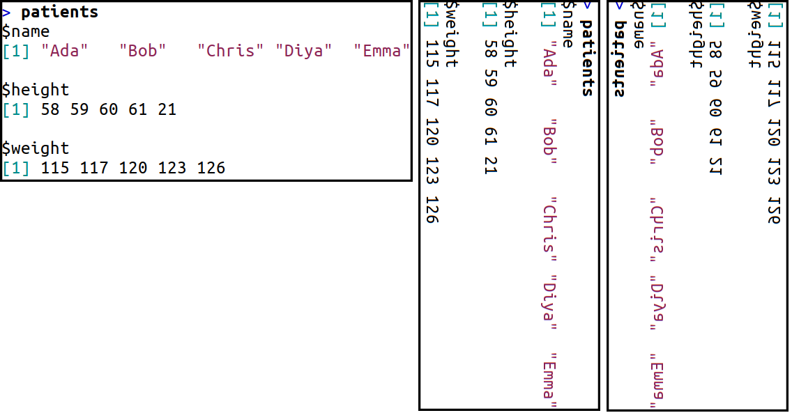
How to transform a list to a dataframe. The list (left) displays exactly the same data as the health example above. In the middle, the list is rotated 90°. At right, the image is also horizontally flipped to preserve the order of columns. Obviously, data frames are printed so that the text is not flipped!
In R, data frames are made of lists (see Section 8) in which each element is a vector of the same length. Each vector represents a column, not a row, and each row of data frame corresponds to the element at a certain position in each of the vectors in the list. You can think of data frame as if you print a list, and then rotate it 90° clockwise. This is why it is important to understand lists when working with data frames.
Through their list origin, data frames can contain variables that are of different type. In the example above, name is character while height is numeric. These are different components of the list. But all names must be character–they are elements of the same vector in the list.
You can work with data frames using the same tools as when working with lists. But data frames include additional properties that are usually more convenient.
12.2 Working with data frames
This section describes the basic functionality of data frames. The most important topic–accessing data in data frames–is described in Section 12.3.
12.2.1 Creating Data Frames
This section shows how to create data frames manually. This is a skill that is rarely used–normally you load data from external sources, such as csv files (see Section 12.5 below). But it comes in handy when you need to debug or test some functionality on data frames.
Data frames can be made with the function data.frame(). As
arguments, you have to provide the variables–data vectors of equal length. Here
is a code that creates the same example patients’ data frame from above:
## create data vectors
name <- c("Ada", "Bob", "Chris", "Diya", "Emma")
height <- 58:62
weight <- c(115, 117, 120, 123, 126)
## combine data vectors into a data frame
patients <- data.frame(name, height, weight)
patients
## name height weight
## 1 Ada 58 115
## 2 Bob 59 117
## 3 Chris 60 120
## 4 Diya 61 123
## 5 Emma 62 126You can see that a data frame is printed as a nice rectangular table, not as a ragged list. This is one of additional properties of data frames.
Because data frames are lists, you can access the values of patients
using the same dollar notation or double-bracket notation as in case
of
lists:
## [1] 115 117 120 123 126## [1] 58 59 60 61 62Exercise 12.3 Create a data frame that contains three variables: country name, its capital’s name, and its population (at least five countries). Choose suitable names for your three variables.
- Now extract country name using the dollar-notation.
- Extract country population using double-bracket notation
- Extract capital using indirect variable name (See Section 8.3.2).
See the solution
12.2.2 Describing Data Frames
One of the first steps you do when you encounter a new data frame is
to get a basic idea what it contains. Here we describe a number of
functions that provide such summary data. A brief summary of the
functions is below (assume df is a data frame):
| Function | Description |
|---|---|
nrow(df) |
Number of rows |
ncol(df) |
Number of columns |
dim(df) |
Dimensions (rows, columns) |
names(df) |
column names |
head(df, n) |
the first n rows (as a new data frame) |
tail(df, n) |
the last n rows (as a new data frame) |
For instance, if we want to know how many rows are there in the patients data frame, we can find it with
## [1] 5The function ncol() behaves in a similar manner. However, dim()
returns bot number of rows and columns–it returns a vector with the
first element being the former and the second element the latter:
## [1] 5 3names() and colnames() are synonyms and return the variable names
of the data frame:
## [1] "name" "height" "weight"You can also give names to rows of data frames. For instance, instead of having a separate column for names, one can put the name as a row name. But currently row names are just row numbers:
## [1] "1" "2" "3" "4" "5"Finally, head() and tail() show a few first and last lines of the
data frame (by default six lines). To show the last two lines you can
do
##   name height weight
## 4 Diya     61    123
## 5 Emma     62    126
There is also an RStudio-exclusive option, View() that opens the
data frame in an RStudio window with a spreadsheet-like interface.
However, you cannot use View() in many contexts. For example, if you
compile your results to an html or pdf file, then the result must be
viewable with a browser or a pdf-viewer, and hence the
RStudio-specific View() will give an error.
Some of these description functions can also be used to
modify
the data frame. For example, you can use the names() to assign new
names to the variables in data:
##    Name Inches Pounds
## 1   Ada     58    115
## 2   Bob     59    117
## 3 Chris     60    120
## 4  Diya     61    123
## 5  Emma     62    126
Note how we assigned new values to the column names, and as a result, the data frame has new variable names.
12.3 Accessing Data in Data Frames
But we cannot use data frames for much unless we are able to manipulate and access these data. First, we discuss perhaps the most important tasks: selecting desired variables and filtering based on certain conditions. Afterwards, we show even more indexing methods.
There is an alternative way of accessing data in data frames–the way of pipes and dplyr. That, a much more intuitive way, is discussed in Section 13.
We use a small data frame of emperors:
name <- c("Qin Shi Huang", "Napoleon Bonaparte", "Nicholas II",
          "Mehmed VI", "Naruhito")
born <- c(-259, 1769, 1868, 1861, 1960)  # negative: BC
throned <- c(-221, 1804, 1894, 1918, 2019)
ruled <- c("China", "France", "Russia", "Ottoman Empire", "Japan")
died <- c(-210, 1821, 1918, 1926, NA)  # Naruhito is alive
emperors <- data.frame(name, born, throned, ruled, died)
emperors
## name born throned ruled died
## 1 Qin Shi Huang -259 -221 China -210
## 2 Napoleon Bonaparte 1769 1804 France 1821
## 3 Nicholas II 1868 1894 Russia 1918
## 4 Mehmed VI 1861 1918 Ottoman Empire 1926
## 5 Naruhito 1960 2019 Japan NANote that as Naruhito is still alive, we do not know his year of death. We use a special value NA (not available) in its place. See more in Section 12.6.
Exercise 12.4
Use the descriptive functions from Section 12.2.2. Find:- What are the column names of the emperors data frame
- How many rows are in the data frame?
- How many columns are in the data frame?
- Print its 2 first lines
- Print its 3 last lines
12.3.1 Selecting variables
Typically, when working with data, one of the most important tasks is to extract certain variables. Data frames make it (relatively) easy in two different ways.
Dollar notation is easier to write: it is just
dataframe$variable. For instance, if we want to pull out emperors’
names, we can ask this as
## [1] "Qin Shi Huang"      "Napoleon Bonaparte" "Nicholas II"
## [4] "Mehmed VI"          "Naruhito"
Remember–data frames are made of lists, and it is the same dollar notation we used for extracting list components in Section 8.3.4.
Double-bracket notation is also similar to that of lists (Section
8.3.2): you put the name (as a string) in double
brackts like dataframe[["variable"]]. So we can exactly the same
vector of
emperors’ names as
## [1] "Qin Shi Huang"      "Napoleon Bonaparte" "Nicholas II"
## [4] "Mehmed VI"          "Naruhito"
The dollar notation is usually easier to write, and hence the double-bracket notation is mainly used for indirect variable names (See Section 8.3.2). For instance:
## [1] "Qin Shi Huang"      "Napoleon Bonaparte" "Nicholas II"
## [4] "Mehmed VI"          "Naruhito"
Exercise 12.5 What happens if you try to use indirect variable names with dollar-notation?
See the solution
This was about extracting individual variables. But the real datasets may contain a large number of columns, most of which we do not need for the particular analysis. So another task we often do when we start to work with a new dataset, is to limit the number of columns to a smaller and more manageable set. It is often easier to work with a smaller “sub-dataframe” than with the huge original dataframe: when printing, less numbers on screen is easier to understand what you need; and if the datasets are large, we may also gain in terms of computing performance and memory usage.
The most obvious approach here is just to list the variable names we want to preserve. For instance, if we are only interested in name and year of birth, we can write
##                 name born
## 1      Qin Shi Huang -259
## 2 Napoleon Bonaparte 1769
## 3        Nicholas II 1868
## 4          Mehmed VI 1861
## 5           Naruhito 1960
Technically, this is almost like list indexing by name (see Section 8.3.2)–the list indexing returns a sublist that only contains the named components. But as emperors is a data frame, it returns a sub-dataframe, not a sublist.
This approach is a good one if we only want to preserve a few
variables and “forget” the others. But other times we only want to
remove a few variables and keep everything else. This can be achieved
by setting those variables to NULL, a special symbol for empty
element. This will remove the component, exactly as in case of lists
(see Section 8.4). We can remove throned variable
as
##                 name born          ruled died
## 1      Qin Shi Huang -259          China -210
## 2 Napoleon Bonaparte 1769         France 1821
## 3        Nicholas II 1868         Russia 1918
## 4          Mehmed VI 1861 Ottoman Empire 1926
## 5           Naruhito 1960          Japan   NA
Note that if the variable does not exist, setting it to NULL is
silently ignored
##                 name born          ruled died
## 1      Qin Shi Huang -259          China -210
## 2 Napoleon Bonaparte 1769         France 1821
## 3        Nicholas II 1868         Russia 1918
## 4          Mehmed VI 1861 Ottoman Empire 1926
## 5           Naruhito 1960          Japan   NA
There are no warnings, and the data frame is unchanged.
We’ll learn more, easier and more powerful methods to select variables in Section 13.
Exercise 12.6 Sometimes you need to do similar tasks with all variables in the data frame. A good way to do it is a for-loop.
Print the column names in the emperors data frame
Write a loop over all columns in your data frame. in the loop, print the column name (use
cat()for printing).Write a loop over all columns in your data frame. In the loop, print the variable name (use
cat()), and the variable itself (useprint()).Write a loop over all columns in your data frame. In the loop, print the variable name (use
cat()), andTRUE/FALSE, depending if the variable is numeric.Hint: use
is.numeric(df$col)to test if the column is numeric.Write a loop over all columns in your data frame. Inside of the loop print the variable name (use
cat()), and its minimum value if the variable is numeric!Hint:
min(df$col)finds the minimum.
See the solution
12.3.2 Filtering rows of data frames
As discussed above, since data frames are lists, it’s possible to
use both dollar notation (data$variable) and double-bracket notation
(data[["variable"]]) to access the data variables. If used in this
way, the results are vectors and hence individual elements can be
accessed as elements in any other vector. For instance, we can
extract names of all emperors who were born before 1800 as
## [1] "Qin Shi Huang" "Napoleon Bonaparte"Here the first dollar-notation epxression, emperors$name, is
a just a vector of names. The second dollar-notation expression, [emperors$born < 1800], is a logical vector where TRUE corresponds to those who are
born before 1800. Needless to say, you can also use double-bracket
notation here instead of one or both of these dollar-notations
if you want to use indirect variable names.
Note that the expression looks somewhat heavy and bloated–the need to
write emperors$ twice seems to be unnecessary, it also makes the
code harder to read. We’ll learn a more intuitive filtering method in
Section 13.3.2.
Exercise 12.7 Extract names of all emperors who died before year 1800
- Do it using only dollar notation
- Use double bracket notation at the first and dollar notation at the second place
- Use solely double bracket notation.
- Explain, what is the
NAyou see there.
See the solution
12.3.3 Using single-bracket notation to extract both rows and columns
12.3.3.1 Basics of the single-bracket-notation
Perhaps the most powerful way to extract information from data frames
is
a variation of single-bracket notation. This
allows you to specify both rows and columns when extracting data.
Here you need to put two index values separated in the brackets and
separate these by a comma (,):
The first index specifies rows and the second specifies columns. The indices should be similar to how you index elements in vectors and lists–they can be numbers, logical values, or names; and you can mix these three types. Underneath a few examples using the emperors’ data from above. As a reminder, the emperors data is
##                 name born          ruled died
## 1      Qin Shi Huang -259          China -210
## 2 Napoleon Bonaparte 1769         France 1821
## 3        Nicholas II 1868         Russia 1918
## 4          Mehmed VI 1861 Ottoman Empire 1926
## 5           Naruhito 1960          Japan   NA
Extract a single element of 2nd row, 3rd column:
## [1] "France"Extract 2nd and 4th row, 3rd column:
## [1] "France" "Ottoman Empire"Extract 2nd and 4th row, variable “died”:
## [1] 1821 1926Extract 2nd and 4th row, variables “name” and “ruled”:
##                 name          ruled
## 2 Napoleon Bonaparte         France
## 4          Mehmed VI Ottoman Empire
Usually, the result of such index operations is a vector, if only a single column was returned, and a data frame, if multiple columns are needed. For instance, the death years of two emperors is a vector, but if we ask both name and the country they ruled, we get a data frame.
We can also ask for all rows or all columns, by just leaving out the corresponding index:
## [1] "China"          "France"         "Russia"         "Ottoman Empire"
## [5] "Japan"## name born ruled died
## 1 Qin Shi Huang -259 China -21012.3.3.2 Certain confusing results
Handling of missing data is somewhat counter-intuitive. For instance, if we extract all emperors who died before year 1:
##            name born ruled died
## 1 Qin Shi Huang -259 China -210
## NA <NA> NA <NA> NAWe’ll see Qin Shi Huang, which is correct. But we also see a line
of NA-s, which seems weird. This is because there is an emperor,
Naruhito, whose year of death we do not know, and hence the logical
index vector is
## [1] TRUE FALSE FALSE FALSE NAThe last element of the vector is NA, and this causes the line of
missings in the outcome. We just do not know if we have another
emperor in the line.27
An easy solution is to use the which() function that converts the
logical vector into a numeric one, marking which elements are true,
and ignoring missings:
## [1] 1or when extracting emperors:
##            name born ruled died
## 1 Qin Shi Huang -259 China -210
Exercise 12.8 Use the emperors’ dataset.
- extract 3rd and 4th row.
- extract all emperors who died in 20th century (all information about them)
- extract name and country for all emperors who died in 20th century
See the solution
Another frequent source of confusion is related to extracting column as a vector and extracting column as a single-column data frame. A column as a vector can be extracted as
## [1] "China"          "France"         "Russia"         "Ottoman Empire"
## [5] "Japan"
while a data frame is
##            ruled
## 1          China
## 2         France
## 3         Russia
## 4 Ottoman Empire
## 5          Japan
Note the difference: the first result is printed as a vector and the latter as a data frame.
Why does a comma cause such a difference? This is because comma between brackets tells R to use the data frame–specific single bracket notation. If there is no comma, we are doing list indexing, and extracting a sublist of a single component. And because the list is a data frame here, we get a sub–data frame with a single column only.
12.3.3.3 Summary
Here is a brief summary of the main tools:
| Syntax | Description | Example |
|---|---|---|
df[row_num, col_num] |
Element by row and column indices | patients[2,3] (element in the second row, third column) |
df[row_name, col_name] |
Element by row and column names | df['Ada','height'] (element in row named Ada and column named height; the height of Ada. patients data does not have row names.) |
df[row, col] |
Element by row and col; can mix indices and names | patients[2,'height'] (second element in the height column) |
df[row, ] |
All elements (columns) in row index or name | df[2,] (all columns in the second row) |
df[, col] |
All elements (rows) in a col index or name, as a vector | df[,'height'] (complete height column as a vector) |
df[col] |
All elements (rows) in a col index or name, as a one-column data frame | df['height'] (data frame containing only height column) |
Take special note of the 4th option’s syntax (for retrieving rows): you still include the comma (,), but because you leave which column blank, you get all of the columns!
# Extract the second row
df[2, ] # comma

# Extract the second column AS A VECTOR
df[, 2] # comma

# Extract the second column AS A DATA FRAME
df[2] # no comma
Extracting more than one column will produce a sub-data frame; extracting from just one column will produce a vector).
12.3.4 Modifying data frames
The previous tools can also be used to modify existing data frames.
For instance, we can set a new variable, “age” to the “patients” data frame using dollar-notation as
##    Name Inches Pounds age
## 1   Ada     58    115  22
## 2   Bob     59    117  33
## 3 Chris     60    120  44
## 4  Diya     61    123  55
## 5  Emma     62    126  66
Instead of adding new variables, we can also overwrite the existing ones in the same way. Here an example about how to use double-bracket notation for replacing “Pounds”:
##    Name Inches Pounds age
## 1   Ada     58    120  22
## 2   Bob     59    120  33
## 3 Chris     60    130  44
## 4  Diya     61    130  55
## 5  Emma     62    140  66
It is also possible to replace only parts of the data frame, for instance, let’s add 10 lb of weight to everyone who is over 40:
##    Name Inches Pounds age
## 1   Ada     58    120  22
## 2   Bob     59    120  33
## 3 Chris     60    140  44
## 4  Diya     61    140  55
## 5 Emma 62 150 66- on both sides of the assignment, we ensure we only work with those
who are over 40 (
patients$age > 40). - on both sides we work only with “Pounds” (
patients$Pounds) - on the right-hand side we add “10” to the Pounds of everyone who is over 40 (there are 3 such patients)
- and finally, on the left-hand side, we assign such new weights to the “Pounds” in the data frame.
This is conceptually similar to vector operations (see Section
6.5). In fact, these are vector operations as
patients$Pounds is a vector!
Finally, the same task can be achieved with ifelse() (see Section
10.3.3):
patients$Pounds <- ifelse(patients$age > 40,
                           # who is over 40?
                          patients$Pounds + 10,
                           # add 10lb to those
                          patients$Pounds)
                           # otherwise keep the weight
patients
## Name Inches Pounds age
## 1 Ada 58 120 22
## 2 Bob 59 120 33
## 3 Chris 60 150 44
## 4 Diya 61 150 55
## 5 Emma 62 160 66This is perhaps more clear that the indexed assignment above. It will become even easier to read when using dplyr tools (see Section 13).
Exercise 12.9 A year has passed and everyone has aged by a year. Add one year to everyone’s age!
Here is some helper code to create data:
Name <- c("Ada", "Bob", "Chris", "Diya", "Emma")
Inches <- c(58, 59, 60, 61, 62)
Pounds <- c(120, 120, 150, 150, 160)
age <- c(22, 33, 44, 55, 66)
See the solution
12.4 R built-in datasets
Above, we created simple data frames manually. R also has a number of built-in data frames, and a number of packages that contain even more data frames. These are designed for testing and demonstration purposes, for actual analysis you usually need to load datasets from disk (see Section 12.5.3).
What is a built-in dataset? All programming languages, including R,
contain certain built-in values. Such values are the constant pi
(3.1416), logical constants TRUE and FALSE, and other similar
values.
In a similar fashion, R also has built-in datasets. Depending on how
they are set up, it may be possible to access those directly, or using
the data() function.
For instance, iris is a built-in dataset about size of iris flowers
(see Section I.13). You can just use it through its
name, iris. Let’s take a quick look:
##   Sepal.Length Sepal.Width Petal.Length Petal.Width Species
## 1          5.1         3.5          1.4         0.2  setosa
## 2          4.9         3.0          1.4         0.2  setosa
## 3          4.7         3.2          1.3         0.2  setosa
it contains five columns, flower size and species. Importantly, from the usage perspective, the built-in dataset is just a data frame, exactly this kind of data frame as what you created manually above.
Not all built-in data are data frames. For instance, state.abb is a
character vector of 2-letter abbreviations of the U.S. states (see
Section I.20):
## [1] "AL" "AK" "AZ" "AR" "CA" "CO" "CT" "DE" "FL" "GA"If datasets are provided by other packages, these can be loaded with
loaded with data()
command. For instance, the ice cream data from Ecdat package
(see Section
I.11) can be loaded
##    cons income price temp
## 1 0.386     78 0.270   41
## 2 0.374     79 0.282   56
## 3 0.393     81 0.277   63
## 4 0.425     80 0.280   68
Another advantage of this approach is that you tell exactly from which package the dataset should be loaded. This is important if multiple packages provide datasets of the same name.
You can learn more about both built-in and package-provided dataset with the command
Exercise 12.10 What is the data structure of the built-in dataset co2? What do the
values represent?
See the answer
12.5 Working with CSV Data
So far you’ve been constructing your own data frames. It is a good skill and a good way to learn to handle data frames, but in practice, such manual coding is rarely needed besides debugging. It’s much more common to load data from somewhere, for instance from a file on your computer or from internet.
12.5.1 CSV file format
While R is able to ingest data
from a variety of sources and in different formats,
this chapter will focus on reading tabular
data in comma separated value (CSV) format, often stored in a file
with an extension .csv.
In this format, each line represents a record
(row) of data, while each feature (column) of that record is
separated by a comma. In csv format, the health data from above
might look like:
Ada,58,115
Bob,59,117
Chris,60,120
Diya,61,123
Emma,62,126
There are a variety of csv file format flavors, another popular option is to separate the columns not by comma but by a tab-symbol. The health data would now look like
Ada 58  115
Bob 59  117
Chris   60  120
Diya    61  123
Emma    62  126
The advantage of tab-separated files is that they are somewhat easier to read by humans. There are many other options, e.g. in languages were comma is the standard decimal separator, it is common to use semicolon to separate columns instead. But despite of the different separators, all those formats are typically (and confusingly) referred to as “comma-separated files” and the character that separates the columns is often called separator or delimiter. Different separators across different datasets is a frequent source of confusion for beginners. It is critical to get the separator right, but fortunately one can usually get the separator automatically detected by computer. Also, wrong separator usually results in very distinct problems that are easy to diagnose.
Spreadsheet programs like Microsoft Excel or Google Sheets can also
load, export and manipulate data that is saved in this format.
However, one cannot save formatting and colors in a .csv file, .csv
format can only handle data.
12.5.2 Where is my file???
One of
the biggest sources of frustration when loading .csv files that beginners
encounter is to tell R where on the computer the data is located.
Normally, you should use relative path to navigate to the data file in
your project. Remember, relative path is relative to the current
working directory (see Section 2.3) and R’s working
directory is normally the one where you set up your project (see
Section 2.2.2 for how to set up projects).
This is perhaps the best way to ensure that you
have a consistent working directory: you set up an RStudio project in
the folder where you are currently working.
In any
case, you can find it out with getwd() command (see Section
11.1).
As the file will be loaded by R, it is fairly obvious that we need to code the path relative to R’s current working directory. Remember–all programs have their working directory for exactly such tasks.
But if, for some reason,
you haven’t created a project, or if you need to
work in a folder outside of the project, you may want to change your
working directory. This can be done with
setwd() command.
This function accepts both relative and absolute path, so you can
change directory both inside of the project (relative) or move, e.g.,
to your desktop (absolute). In general, it is advisable to avoid
using setwd() inside of scripts, as people usually do not expect
scripts to change directories.
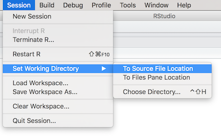
Changing working directory through RStudio menus.
Another way to change the working directory is through the RStudio menus, namely Session -> Set Working Directory. You can either set the working directory To Source File Location (the folder containing whichever script you are currently editing; this is usually what you want), or you can browse for a particular directory with Choose Directory.
It is normally enough to set working directory once per session. The next important thing is to understand what is the relative path of your data file and how to load it.
12.5.3 Loading csv files
There are multiple ways to load csv files into R. The base-R includes
functions (among others) read.csv() for reading comma-separated
files and read.delim() for reading tab-separated files. Below, we
focus on read_delim() in package readr that will automatically
detect the correct separator.
readr is a separate package that needs to be installed (using
install.packages("readr")) and thereafter loaded using
library(readr).
See Section 5.6
for more about how to install and load packages.
readr is also part of tidyverse
(see Section 13.3), so if you have
installed and loaded the latter, there in no need to load readr
separately. We will start using tidyverse later.
The difference between read_delim() and read.delim() is a frequent
source of confusion:
read_delim()detects the correct delimiter automatically (normally either tab or comma)read.delim()assumes that it is tab, and does not read the file correctly if it is comma
In this book we only use read_delim().
read_delim() reads the given csv file and returns its content as a
data frame. It will automatically figure out the correct separator,
but you can also specify it manually in case the automatic detection
fails. It can read compressed files, often ending with .csv.bz2 or
.csv.bz so if you have such a file, there is no need to decompress
it.
Normally you want to assign its returned data frame to
a variable (otherwise
it will be just printed and forgotten). Typical usage, reading data
from file.csv and storing it into workspace variable data looks
like:
Let’s load a tiny height-weight data from directory data inside of the current working directory. If you want to replicate this exercise, you should either download the dataset into the same folder, or adapt the path in the command below.
This function will return a data frame, and we save it into variable hw.
Note how the file name now is specified not just as file name but as
relative path: "data/height-weight.csv" means to first go into a
folder data (inside the current working directory),
and thereafter grab the file height-weight.csv from
there. If you are unsure if your current working directory contains
the folder data, then you should check
- what is your current working directory? (
getwd()) - what are the files and folders there as R sees them?
(
list.files())
When reading is successful, then read_delim() reports a few basic
facts about the file. Here we see that it contains 5 rows
and
4 columns. We also see that it’s delimiter is tab–"\t"
is the tab symbol, and it contains one string variable (sex), and
three numeric variables (age, height, weight; dbl, double,
stands for numeric variables).
Finally, now we can also print the dataset:
## # A tibble: 5 × 4
##   sex      age height weight
##   <chr>  <dbl>  <dbl>  <dbl>
## 1 Female    16    173   58.5
## 2 Female    17    165   56.7
## 3 Male      17    170   61.2
## 4 Male      16    163   54.4
## 5 Male      18    170   63.5
A note about file paths on Windows. R supports the unix-style forward
slashes / as path separators, i.e. you can always
write "data/file.csv". On
windows, one can also use windows-standard backslashes \. However, as
backlash is also an escape character inside of strings, these must be
written as double backslashes: "data\\file.csv". In this book we
use forward slash as path separator.
See also Section 21.1.2 for raw strings.
12.5.4 Troubleshooting loading files
The two common problems the beginners face when loading data are using wrong file path and using wrong separator. Here we discuss a few ways to understand and fix these problems.
If you get the file path wrong then you’ll see an error message like
## Error: 'non-existent-file.csv' does not exist in current working directory ('/home/siim/tyyq/info201-book').The error message tells exactly what the problem is: the file non-existent-file.csv does not exist where you are looking at it. Unfortunately the error alone is not enough to suggest a solution. But here are a few steps your should take.
- Ensure you understand the file system tree and the relative path (see Section 2.1).
- Make sure you know where did you put the file. Is it in fact in the place you think it is? Note that some computers may have multiple Desktop folders, and you may be looking at the wrong one!
- What is the current working directory of R? Use
getwd()to find it out. Is the relative path of the file with respect the current working directory correct? - Is the file name correct? You may have mis-spelled it, or there
may be an extension that is normally hidden in the graphical file
viewer. (
list.files()on console always shows the full file name.)
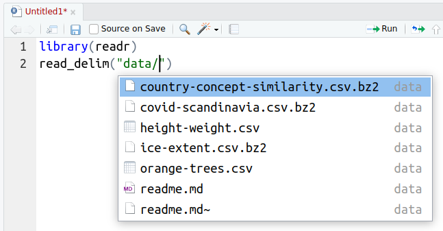
File name completion at work: hitting TAB-key in rstudio when writing
the file name will give you a menu of suggested files.
We strongly recommend that you learn to use the file name completion
feature in RStudio: each time you need to write the file name, start
with writing a few first letters and hit the TAB key.
RStudio will either
auto-complete the name (if there is only a single option), or give you
a menu of suggestions if there are more. This not just lessens your
typing burden, but it also ensures that the path is correct and there
are no typos in the file name. And remember: if you want to go up
in the file system tree, you can start with "../" and then hit the
TAB-button.
You may achieve similar tasks as RStudio’s file name completion by using R commands as well. For instance, to view files in the “data” folder, you can issue command
##  [1] "alcohol-disorders.csv"              "country-concept-similarity.csv.bz2"
##  [3] "covid-scandinavia.csv.bz2"          "csgo-reviews.csv.bz2"
##  [5] "emperors.csv"                       "emperors.csv~"
##  [7] "fatalities.csv"                     "height-weight.csv"
##  [9] "ice-extent.csv.bz2"                 "orange-trees.csv"
## [11] "readme.md"                          "readme.md~"
## [13] "titanic.csv.bz2"                    "ukraine-oblasts-population.csv"
## [15] "ukraine-with-regions_1530.geojson"
You’ll receive a character vector of all files that R found in the folder “data/”. And importantly–you’ll see them in the exact same way as R sees them. This includes the path relative to the current R working directory. See Section 11.2 for more details.
Another common problem is to use a wrong delimiter. read_delim()
will normally get it right, but not always. Also, a web search may
give you different suggestions, e.g. read.csv() that has different
assumptions about the delimiter (it assumes it is comma). Here is an
example what happens when we get the separator wrong. We use
read.csv() that assumes the columns are separated by commas:
## [1] 5 1Firstdim() tells us the right number of rows (5) as the
separators do not mess up lines. But number of columns–1–is clearly
wrong. This is because read.csv() is expecting to see commas that
separate columns, but as it cannot find any, it lumps all values into
a single column.
When looking at data
##   sex.age.height.weight
## 1 Female\t16\t173\t58.5
## 2 Female\t17\t165\t56.7
## 3   Male\t17\t170\t61.2
## 4   Male\t16\t163\t54.4
## 5   Male\t18\t170\t63.5
we can see a repeated pattern of \t present in it. This is the tab
symbol (in a string, you mark tab symbol as "\t"). This also gives
a strong hint that data was loaded with a wrong separator, and the
correct one is tab. So you should use read.delim() (this assumes
the separator is tab), or just read_delim() that can detect the
separator automatically.
A csv file may look like
Ada,58,115
...
(comma-separated) or
Ada 58  115
...
(tab-separated).
separator or delimiter is the character that is used to separate data columns in csv file. It is typically comma or tab.
Loading files: use
read_delim(path)(a function in readr or tidyverse package) loads the file and detects the correct delimiter.read.delim()will not detect the correct one!
12.6 Learning to know your data
Data is treacherous. There are many things that can go wrong when working with data, and before you even start any serious work, you should have an overview of what exactly is there in the dataset. Below, we describe a few things that you should do each time you start working with a new dataset.
12.6.1 Did you load data correctly?
You first task should be to check if you loaded data correctly–and if you loaded the correct dataset. For instance, if you want to analyze Titanic data, you ought to load it along these lines:
But what exactly did you load? Maybe read_delim() was not the right
way to load this file? Maybe the file got corrupted somehow? Maybe
titanic.csv is not the file you want in the first place? Let’s
check!
Perhaps the first and simplest way to check the dataset is just to print its dimension (rows and columns):
## [1] 1309 14This looks encouraging: 1309 rows and 14 columns feels about right for a passenger list data. But this was about rows and columns–we still do not know what do these contain. I recommend to test it with printing a few lines of data to have a visual idea what is there:
## # A tibble: 3 × 14
##   pclass survived name                           sex       age sibsp parch ticket
##    <dbl>    <dbl> <chr>                          <chr>   <dbl> <dbl> <dbl> <chr>
## 1      1        1 Allen, Miss. Elisabeth Walton  female 29         0     0 24160
## 2      1        1 Allison, Master. Hudson Trevor male    0.917     1     2 113781
## 3      1        0 Allison, Miss. Helen Loraine   female  2         1     2 113781
##    fare cabin   embarked boat   body home.dest
##   <dbl> <chr>   <chr>    <chr> <dbl> <chr>
## 1  211. B5      S        2        NA St Louis, MO
## 2  152. C22 C26 S        11       NA Montreal, PQ / Chesterville, ON
## 3  152. C22 C26 S        <NA>     NA Montreal, PQ / Chesterville, ON
It is convenient to check the first few lines with head(), but
sometimes the beginning of datasets looks good, while further down it
is empty or garbled. In that case a random sample may give you a
better idea.
## # A tibble: 3 × 14
##   pclass survived name                            sex      age sibsp parch ticket
##    <dbl>    <dbl> <chr>                           <chr>  <dbl> <dbl> <dbl> <chr>
## 1      3        0 Brocklebank, Mr. William Alfred male      35     0     0 364512
## 2      3        1 McDermott, Miss. Brigdet Delia  female    NA     0     0 330932
## 3      1        0 Kent, Mr. Edward Austin         male      58     0     0 11771
##    fare cabin embarked boat   body home.dest
##   <dbl> <chr> <chr>    <chr> <dbl> <chr>
## 1  8.05 <NA>  S        <NA>     NA Broomfield, Chelmsford, England
## 2  7.79 <NA>  Q        13       NA <NA>
## 3 29.7  B37   C        <NA>    258 Buffalo, NY
Currently, both of these functions show a similar picture. And this picture is plausible–you see columns with reasonable names, and meaningful values. It is fine if you do not understand all of these–at least they look plausible. It is also fine if some values are missing–most datasets contain many-many missing values.
But what happens if something goes wrong with data loading? Obviously, this depends on what exactly is wrong. If you have accidentally deleted your dataset then you may see a “no such file” error. If the dataset is empty, you may find that your data frame contains zero rows. Here is an example what happens if you load it with wrong delimiter (see also Section 12.5.4):
## [1] 1309 1This will issue the first warning: the dataset contains a single column only. A single column is not necessarily wrong, but if you have a slightest idea about your dataset, you should be able to tell whether it makes sense.
Next, printing a few lines shows:
##                            pclass.survived.name.sex.age.sibsp.parch.ticket.fare.cabin.embarked.boat.body.home.dest
## 1                              1,1,Allen, Miss. Elisabeth Walton,female,29,0,0,24160,211.3375,B5,S,2,,St Louis, MO
## 2 1,1,Allison, Master. Hudson Trevor,male,0.9167,1,2,113781,151.5500,C22 C26,S,11,,Montreal, PQ / Chesterville, ON
It shows that the data is there, just not correctly arranged into columns.
Finally, we may also check names of the mis-read dataset:
## [1] "pclass.survived.name.sex.age.sibsp.parch.ticket.fare.cabin.embarked.boat.body.home.dest"Again, all names are there, but they are combined into a single
column. Here these problems are caused by read.delim() that assumes
the columns are separated by tab, while in fact they are separated by
comma.
12.6.2 Data types
After the data is correctly loaded, you probably want to take a quick look at column types. We discussed the basic types–numbers, texts, and similar in Section 4.4. But there are more data types, e.g. dates and timestamps (see Section 15.3), categorical data (see Section 21.2), and others. It is helpful to see, if the column types are what you might expect.
An easy way to see the data types is just to print a few lines of the dataset. The printout will include the abbreviated column type:28
## # A tibble: 1 × 14
##   pclass survived name                          sex      age sibsp parch ticket  fare
##    <dbl>    <dbl> <chr>                         <chr>  <dbl> <dbl> <dbl> <chr>  <dbl>
## 1      1        1 Allen, Miss. Elisabeth Walton female    29     0     0 24160   211.
##   cabin embarked boat   body home.dest
##   <chr> <chr>    <chr> <dbl> <chr>
## 1 B5    S        2        NA St Louis, MO
We can see that pclass is of type dbl (“double”, i.e. a “double-precision” number), name is chr (“character”, i.e. text), and so on.
Exercise 12.11 What do you think, why is type of the boat above “chr” (text), not number, although its value is the number “2”? Are the ticket, fare, and cabin data types what you expect?
Understanding the data types will help to spot problems in the data. For instance, age is currently a number (“dbl”). This is probably what we might expect–when talking about “age”, we usually mean age in years. But what if age turns out to be text (“chr”)? How might that happen? This may indicate problems with coding–the column contains values that cannot be converted to a number. For instance, someones age may be listed as “middle-aged”, “twenties” or “younger than 50”. Alternatively, there may just be typos or other errors in the column, e.g. age may be listed as “4t” or as “male”. The former is probably a typo, the latter probably means that someone has entered sex into the wrong column.
You need to know the data type before we do any computations. Otherwise, you may get surprising results, e.g. you may learn the someone in their twenties is older than a 50-year old 🙄
## [1] "twenties"In case you cannot or do not want to print the few lines of data as
above, you can use the function class(). For instance, let’s load
the Steam CS-GO data:
## [1] "rating"       "nHelpful"     "nFunny"       "nScreenshots" "date"
## [6] "hours"        "nGames"       "nReviews"
We can manually see that both rating and date are text:
## [1] "character"## [1] "character"If you want to know the type of all columns, then you can use a for-loop:
## rating: character
## nHelpful: numeric
## nFunny: numeric
## nScreenshots: numeric
## date: character
## hours: numeric
## nGames: numeric
## nReviews: numeric
Or better, sapply() (see Section 20.2.1):
##       rating     nHelpful       nFunny nScreenshots         date        hours
##  "character"    "numeric"    "numeric"    "numeric"  "character"    "numeric"
##       nGames     nReviews
##    "numeric"    "numeric"
Exercise 12.12 Write a for loop over all columns of the csgo data frame. Print out the average value for the columns, but only for those columns that are numeric!
12.6.3 Missing values
After you have seen that you loaded the data correctly, you may want to check how much information is there in data. One of the persistent problems with real-world data is missing values. Missing values are normally displayed as NA (for “Not Available”), no matter for what reason the data is missing. It may be missing because it is not applicable for a given case (e.g time of death of a living person, see Section 12.3), or it may be that the information exists but we do not know it, or it may be that whoever created the dataset just forgot to enter it. It may also caused by errors in data pre-processing code.
R has a dedicated function, is.na(), that takes in a vector and
returns a logical vector, True if the element is missing and False
if it is not. For instance,
## [1] FALSE FALSE TRUE FALSE TRUEAs you see, elements 3 and 5 are True (they are missing) while the others are False (they are valid values).
We can use it to count the number of missings (see Section 6.6):
## [1] 2or the percentage of missings:
## [1] 0.4We can also remove missings from x as
## [1] 1 2 4Note what happens here: first we invert the meaning of is.na() with
the logical NOT ! and get
## [1] TRUE TRUE FALSE TRUE FALSEi.e. True corresponds to non-missing elements and False to missing elements. And thereafter we use logical indexing (see Section 6.4.3) to extract only non-missing elements.
Exercise 12.13 Create a data frame with two columns: one of these is the x above with two missing values. The other column should not contain any missings.
Extract only those rows from the data frame that do not contain missings.
Before any further analysis, you want to check how many missings is there in the variables you want to use in your analysis. For instance, assume you want to use variables age, survived, and boat in the titanic dataset. You may compute
## [1] 263to see that there are 263 missing age values. Or alternatively,
## [1] 0.6287242indicates that a very large percentage of boat is missing, casting doubt if it can be used for any analysis at all.29
12.6.4 Range and implausible values
Unfortunately, not all missing values are coded as NA. First, it is
a common habit in many survey datasets, but also elsewhere, to denote
missing values with certain implausible numbers, e.g. “-1” or “999”.
These numbers do not show up with is.na() because, well, they are
valid numbers! I stress here that they are valid numbers, not
necessarily valid ages, ticket prices or whatever the variable is describing.
There are two good strategies to assess such problems.
First, one should look up the data documentation. If the dataset is carefully designed and coded, the documentation will probably tell what values have special meaning.
Example 12.1
World Value Survey asks many questions like “How important is family in your life” with answer ranging from “1” (very important) to “4” (not at all important). But the interviewer is also told to use negative numbers as- -1: don’t know
- -2: no answer
- -3: not applicable
These are missing values–we do not know how important is family if we
get no answer. But these are valid numbers and hence not picked up by
is.na().
But too often, the documentation is incomplete or missing altogether, and you are left to guess what certain values mean. In that case, a good option is to look at maximum and minimum values (for numeric data), or to find all text values there (if categorical data). For instance, let’s analyze the age in Titanic data. We can guess it is passengers’ age in years, but is it? What is its minimum value:
## [1] NAWhy is minimum value missing? This is because some age values are
missing, and hence we do not know what is the true smallest age.
This is a good but annoying way to remind us that we cannot
compute the minimum value of data that contains missings.
Fortunately, an easy workaround is to set the argument na.rm to
True:
## [1] 0.1667na.rm = TRUE tells R to ignore missing values when computing the
minimum. The maximum age value works in the similar fashion, one can
also use range() that prints both minimum and maximum age value:
## [1] 0.1667 80.0000This indicates that the youngest passenger was 2 months, and the oldest one 80 years old. Both are plausible values and so we can conclude that all passenger age values are plausible in Titanic data–they all must be in the range from 2 months till 80 years.
Exercise 12.14
Load Ice extent data. Let’s focus on ice extent (column extent) and area (area).Do these columns include any missing values (NA-s)?
What is a plausible range for ice extent and area? Can you suggest a lower bound and an upper bound that the ice extent/area plausibly cannot exceed?
You may need to consult the documentation in Section I.12 to understand these variables.7
Are all extent and area values plausible? Explain what do you see!
If the column we are interested is categorical, then we cannot just
compute the minimum and maximum of it. If possible, then one should
look at all values that are there. This can be done with unique()
(that displays all unique values), or table(), that also shows how
many times each value occurs in data.
Let’s take a look at the boat column in Titanic data:
##  [1] "2"       "11"      NA        "3"       "10"      "D"       "4"       "9"
##  [9] "6"       "B"       "8"       "A"       "5"       "7"       "C"       "14"
## [17] "5 9"     "13"      "1"       "15"      "5 7"     "8 10"    "12"      "16"
## [25] "13 15 B" "C D"     "15 16"   "13 15"
The result contains a number of boat names (boat numbers). It also contains NA for missing boat. Importantly, it also contains a few examples where an individual has been assigned multiple boats, such as “13 15 B”. I do not know what it means. It is possible that someone was transferred from one boat to another, but this is unlikely. Maybe the data collectors just weren’t sure which boat the passenger was in.
The table() function will give a broadly similar picture, but
importantly, it also tells the frequency of these values:
##
##       1      10      11      12      13   13 15 13 15 B      14      15   15 16
##       5      29      25      19      39       2       1      33      37       1
##      16       2       3       4       5     5 7     5 9       6       7       8
##      23      13      26      31      27       2       1      20      23      23
##    8 10       9       A       B       C     C D       D
##       1      25      11       9      38       2      20
The result may look a little hard to understand at first because it may be unclear where are the boat names and where the corresponding counts. But it contains pairs of rows–the boat names in the upper row and the respective counts in the lower row. For instance, boat “1” was assigned to 5 passenger, boat “10” to 29, and so on. From the table we can see that there are only 7 problematic multi-boat cases (two for “13 15”, 1 for “13 15 B” and so on). Hence we can conclude that by far the most case include valid boat names.
Exercise 12.15 Analyze the home/destination column of Titanic data (home.dest). Do you see implausible values? Missing values? How many different values do you have? Do you think this approach–checking the individual values–is a good way to go here?
Exercise 12.16 When you count the number of different values, you’ll find that
unique() and table() give you a slightly different number:
## [1] 28## [1] 27Which value is missing from table()? How can you include all the
values in the table (see the documentation).
12.6.5 Descriptive analysis
12.6.5.1 Statistical functions
TBD: mean(na.rm=TRUE)
There is also a handy function summary() that displays a few summary
information for vectors, including the number of missings:
##    Min. 1st Qu.  Median    Mean 3rd Qu.    Max.    NA's
##   0.000   7.896  14.454  33.295  31.275 512.329       1
summary() a good way to get a quick overview of individual columns.
In code we usually prefer single values though and then it makes more
sense to use dedicated functions like min(), max() and mean().
12.6.5.2 Largest and smallest values
It is easy to find the maximum fare by using the max() function:
## [1] 512.3292But sometimes it is not all we want–we want to know who was the person how paid that fare. The maximum value is clearly not enough. In that case there are two options:
First, you can use a trick: the logical vector fare == max(fare)
will return TRUE for only those persons who paid the maximum
price, and hence we can extract only those lines:
## # A tibble: 5 × 14
##   pclass survived name
##    <dbl>    <dbl> <chr>
## 1      1        1 Cardeza, Mr. Thomas Drake Martinez
## 2      1        1 Cardeza, Mrs. James Warburton Martinez (Charlotte Wardle Drake)
## 3      1        1 Lesurer, Mr. Gustave J
## 4      1        1 Ward, Miss. Anna
## 5     NA       NA <NA>
##   sex      age sibsp parch ticket    fare cabin       embarked boat   body
##   <chr>  <dbl> <dbl> <dbl> <chr>    <dbl> <chr>       <chr>    <chr> <dbl>
## 1 male      36     0     1 PC 17755  512. B51 B53 B55 C        3        NA
## 2 female    58     0     1 PC 17755  512. B51 B53 B55 C        3        NA
## 3 male      35     0     0 PC 17755  512. B101        C        3        NA
## 4 female    35     0     0 PC 17755  512. <NA>        C        3        NA
## 5 <NA>      NA    NA    NA <NA>       NA  <NA>        <NA>     <NA>     NA
##   home.dest
##   <chr>
## 1 Austria-Hungary / Germantown, Philadelphia, PA
## 2 Germantown, Philadelphia, PA
## 3 <NA>
## 4 <NA>
## 5 <NA>
This will list all the persons who paid as much as the maximum value.
If you are unhappy with the NA-line, then you may add which() (see
Section 12.3.3.2):
## [1] 50 51 184 303and the passengers are
titanic[which(titanic$fare == max(titanic$fare, na.rm = TRUE)),
        c("pclass", "survived", "name", "sex", "age")]
## # A tibble: 4 × 5
## pclass survived name
## <dbl> <dbl> <chr>
## 1 1 1 Cardeza, Mr. Thomas Drake Martinez
## 2 1 1 Cardeza, Mrs. James Warburton Martinez (Charlotte Wardle Drake)
## 3 1 1 Lesurer, Mr. Gustave J
## 4 1 1 Ward, Miss. Anna
## sex age
## <chr> <dbl>
## 1 male 36
## 2 female 58
## 3 male 35
## 4 female 35Alternatively, you can use the function which.max(). This does
not tell the maximum value, but its index, i.e. at which position
is the maximum value in the vector. We can just extract the
corresponding row from the data frame:
## [1] 50## # A tibble: 1 × 14
## pclass survived name sex age sibsp parch ticket
## <dbl> <dbl> <chr> <chr> <dbl> <dbl> <dbl> <chr>
## 1 1 1 Cardeza, Mr. Thomas Drake Martinez male 36 0 1 PC 17755
## fare cabin embarked boat body
## <dbl> <chr> <chr> <chr> <dbl>
## 1 512. B51 B53 B55 C 3 NA
## home.dest
## <chr>
## 1 Austria-Hungary / Germantown, Philadelphia, PAAs you see, both approaches work, but they are also different. fare == max(fare) lists all passengers who paid that much (plus another
row for missing values). which.max() only lists the first such
passenger.
There are also other ways, e.g. by sorting the data frame by price
paid, and then displaying only the first few rows.
See Section 13.3.4 and rank() (Section
13.6.1.3)
for other, more intuitive
approach to find the largest and smallest rows.
Exercise 12.17 Find the youngest passenger on titanic.
12.6.6 Making simple plots
A powerful tool to understand data is to visualize it. Later (Section 14) we will learn about ggplot2 library that is designed for plotting data. Here we will give a brief overview of base-R plotting functionality that is simpler, but may need more work to create plots that git to our needs.
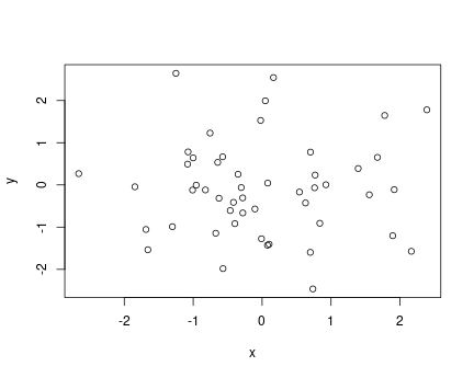
Example scatterplot of 50 random points
The central function in base-R plotting is plot(). It normally
takes two arguments, \(x\) and \(y\), and makes a scatterplot of the \((x, y)\) pairs. Here is an example using random numbers:
This creates a simple scatterplot of 50 points, marked as empty circles. But note that the labels are just the variable names, it also does not have title or explanation. All those must be adjusted or added manually if desired.
plot() function supports a plethora of additional arguments that can
be used for adjusting and customizing the plot. See the example
below.
These include:
xlab,ylab: \(x\) and \(y\)-axis labels. Defaults are the variable names, but frequently those need to be adjusted.main: main title, a text put above the plot in bold font.col: color of the objects (dots in the previous example). It can be a numbered color (1is black,2is red, and so on), a simple color as string (e.g."red"or"green"), it can be a complex R color (e.g."cornsilk2"or"orangered3", see e.g. this image or just google “r colors”). It can also be hex color code, e.g."#998877". There are more options, check out functionsrgb(),hsv()and others.pch: point type.1, the default draws empty circles,2crosses,16filled circles. You can see them withplot(1:20, pch=1:20).lwd: line width for line plots.lwd=1, is the default,lwd=2makes thick lines,lwd=0.5makes thin lines. You can experiment with different numbers.cex: size of the points. Default iscex=1, trycex=2for large points
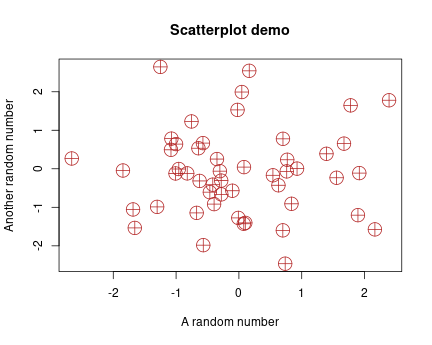
Example of tuned scatterplot
Here is a tuned example of the previous plot:
plot(x, y,
     main = "Scatterplot demo",
     xlab = "A random number",
     ylab = "Another random number",
     pch=10, cex=2.5, col="firebrick")
We use large reddish crossed circle–shaped dots and custom labels.
Another very important option for plot() function is type. This
tells the plot type with "p" (default) meaning points (scatterplot), "l"
meaning line plot, and "b" meaning both points and lines. It is
probably a bad idea to connect these random points with lines, but
line plots have its place for displaying, e.g. time series data.
Exercise 12.18 Why is it a bad idea to make a line plot of random dots? Use
type="l" in the previous example to find it out!
See the solution
We demonstrate this with beavers data, built-in data beaver1 (see Section 12.4). It measures body temperature of a beaver over a day, it looks like
##   day time  temp activ
## 1 307  930 36.58     0
## 2 307  940 36.73     0
## 3 307  950 36.93     0
It contains four variables–date, time, body temperature (°C) and
activity status (“0”: in its nest, “1”: outside). See ?beavers for
more details.
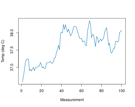
We can see how the body temperature changes over time between 37° and
38°. Note that we have done some plot tuning here: specified
color 3 (green), made the line a bit wider, and adjusted the labels.
Base-R offers a simple way to save plots. Normally, plots are displayed on screen (this is the “default device”). But you can pick a different “device”, e.g. a pdf file. One can save the pdf of the figure as
pdf("plot.pdf", width=6, height=4)  # width, height in inches
plot(...)  # do your plotting here
dev.off()  # finish the pdf file.
Instead of pdf, you can also save png, jpg and other file formats and
supply many other options. See ?pdf and ?png for more
information.
There are three things to be aware of:
- The order of tasks is this: a) open the device (e.g.
pdf()); b) do your plotting; c) close the device (dev.off()). If you do plotting first, you’ll get an empty file as the plot was still done on screen. dev.off()is needed. If you leave this command out, the file will be incomplete and will probably not display. This is the command that ensures the image is completely written to the file.- The plot, including its fonts and point sizes, will be fitted to the image on disk. It typically has different dimensions than what you have on screen, and hence you may be surprised to see fonts and lines that are too large or too narrow. You can either adjust the image size when writing the file, or the font/point/line sizes when doing the plotting.
Finally, ggplot (Section 14) provides an extended functionality to save plots but it still supports the base-R devices as described above.
The need for rectangular structure is suitable for many tasks, but not for all tasks. For instance, if different patients have different number of measurements, then data frames may not be the best way to represent data.↩︎
It may sound counter-intuitive that the computer does not know whether Naruhito–who is alive in 2023–died before year 1. We know that this is impossible. But computers know nothing, unless we explain it to them. And we haven’t explained it.↩︎
Strictly speaking, this is only true for the tibble-flavor of the data frames. Tibbles are the data frames that are loaded with
read_delim(), you can also create them manually. Butdata.frame()function does not create tibbles.↩︎Here it is actually not a problem with data. The reason that boat is missing for over 60% of entries is the sad fact that over 60% of passengers did not get into a boat.↩︎