Chapter 5 Re-using your code: loops and functions
In the previous section we discussed how to use variables, do simple computations, and print the results. This is all useful knowledge. But it is not enough. What if we want to do similar calculations over and over again, each time using slightly different values? We can, obviously, write similar code over and over again, but that is a little stupid thing to do: first, it is tedious; second–each new line of code is a source of additional errors; and finally–if you want to change the way you perform the calculations then you have to change all these lines. Again, it is tedious and error-prone.
Here we’ll discuss two widely used constructs–for loops and functions. Both of these let you to easily re-use your existing code, but in different ways. First, we consider loops and thereafter functions. Functions will be introduced in an abstract sense, followed by an overview of built-in R functions and packages, and finally we explain how to write your own functions.
5.1 For-loops: repeating code
For-loop is one of the simplest ways to re-use the code. It is also a very old programming construct and has been around since 1950-s, see e.g. the Wikipedia page for it.
5.1.1 Repeating commands
Let’s start with a simple example. Let’s say you want to print the squares of numbers from one to five in a form
1^2 = 1
2^2 = 4
...
One such line can be printed with cat() command (see Section
4.5) as
## 2^2 = 4First we use variable i to hold the value, square of which we want to
compute. Thereafter we compute the result, variable i2, equal to
\(2^2\). And finally we print using cat() where we provide it with
five arguments: first the
number, square of which we want to compute (i), thereafter the
constant text where nothing changes (^2 =), and third, the result
(i^2). This is followed by new line ("\n") and finally sep=""
tells not to add extra spaces between the items to be printed.
Now obviously we can repeat the lines above for 5 times. But fortunately, there is an easier way to do it:
## 1^2 = 1
## 2^2 = 4
## 3^2 = 9
## 4^2 = 16
## 5^2 = 25
## doneThis is for loop. It is fairly obvious what it does: it “loops
over” numbers from “1” to “5”, each time setting the variable “i”
equal to that number. And thereafter it computes i2 = i^2 and
prints both i and i2.
Note the necessary changes we made here:
- the second (computing) and third line (printing) are exactly the same as above. No changes here.
- the original first like,
i <- 2is gone, and replaced by the for loop headerfor(i in 1:5). You can imagine it is a series of similar assignments,i <- 1,i <- 2,i <- 3, and so on. - the most important lines of code–for loop body, are inside
curly braces
{and}. The braces should start immediately after the for loop header. Everything that is inside of the braces will be repeated five times, what is outside of braces (printing “done”) is only done once.
Note also that inside of the for-loop body, the variable “i” takes values 1, 2, 3, …, one after the other. It is still the same variable, just the values change inside of the loop.
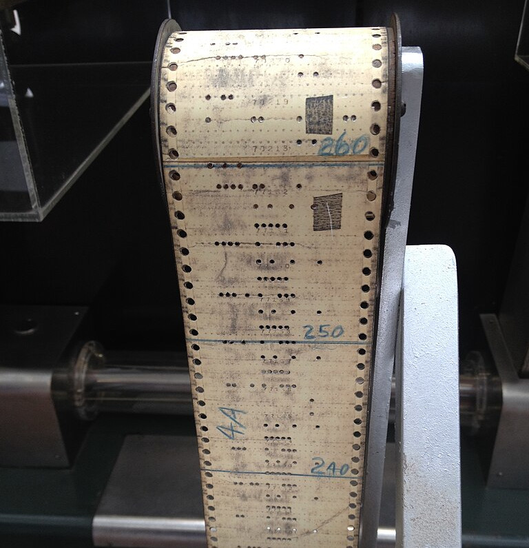
Punched tape for programming Mark-1.
ArnoldReinhold,
CC BY-SA 3.0,
via
Wikimedia Commons
The first digital computer, Mark-1 (built 1943), did not have for-loops, so the commands had to be punched on the paper tape multiple times over. In order to avoid this, the operators sometimes glued the ends of the tape together, in this way creating a long paper loop. There were even special racks and pulleys, to keep the very long loops in place!17
Below is a selection of for-loop related exercises. These are training algorithmic thinking for beginners.
Exercise 5.1 The expression 1:5 is a shorthand for seq(1, 5). seq() is a
function that creates sequences. Look up it’s help by ?seq (on the
console), and use it to modify the loop above in a way that it prints not
numbers 1,2,3,4,…; but only odd numbers 1,3,5,9 (and their squares).
See the solution
Exercise 5.2 Use for-loop to print the following:
7*10 = 70
7*9 = 63
7*8 = 56
...
7*0 = 7
See the solution
Exercise 5.3 Use for-loop to print 10 caret signs like
^^^^^^^^^^Do this by printing just one caret sign at time.
See the solution
Exercise 5.4 Use two for-loops inside each other (nested loops) to print “asivärk”:
^
^^
^^^
^^^^
^^^^^
^^^^^^
^^^^^^^
^^^^^^^^
^^^^^^^^^
^^^^^^^^^^
(The number of signs in row runs from 1 to 10)
See the solution
Exercise 5.5 Write a loop that creates inverted ``asivärk’’:
||||||
|||||
||||
|||
||
|
See the solution
Write a loop that combines the inverted and the normal asivärk:
||||||o
|||||oo
||||ooo
|||oooo
||ooooo
|oooooo
See the solution
Exercise 5.6 Write a loop that creates “wide asivärk”: each line contains two more “o”-s than the previous line:
o
ooo
ooooo
ooooooo
ooooooooo
ooooooooooo
ooooooooooooo
See the solution
Exercise 5.7 Use loop to create “Mountain in rain”:
|||||||o|||||||
||||||ooo||||||
|||||ooooo|||||
||||ooooooo||||
|||ooooooooo|||
||ooooooooooo||
|ooooooooooooo|
See the solution
Exercise 5.8 Use loops to write code that produces the following number pattern:
1  2
3  4
5  6
7  8
9 10- Numbers in the same line should be separated by a space, you also need a line break to get the intended output.
- Do not hardcode the answer–do not write like
cat("1 2")
5.1.2 Accumulating values
Another common task that can be done with for-loops it to accumulate values. Accumulation means to collect all values together, either by just collecting them, or maybe adding or multiplying, or doing something else instead. You can imagine gathering berries–this is a version of accumulation using a for-loop!
Take an empty basket
for(all berries you can see) {
   pick the berry
   put it in basket
}
Now you have all berries in basket.
This example demonstrates all the tools you need to accumulate values. Perhaps the central construct here is the for-loop: for every berry you see, you need to perform the same operations: first pick it up, and then drop it in the basket. Second, you need an accumulator. In the example it is a basket. Also, you want the basket to be empty–it should not contain mushrooms, or dirty socks! But “empty” may mean different things for different tasks, e.g. your basket should be empty and clean for berries, but if you want to add numbers, then it should be “0” instead. Finally, you also need to consider what operation you need for accumulating–when picking berries, you just drop them in the basket, but when adding numbers, you need to use the “+”-operator.
Exercise 5.9 You are going to pick apples. But you do not have any basket, and you can only carry three apples in hand. So you want to take three best apples. How would you write the instructions, like the berry picking ones above, for this case?
- The for-loop need to walk over all numbers from 1 to 10, so we can
just write
for(n in 1:10) { ... }. - What should be the accumulator? As we are “adding the numbers”, we are implicitly asking for the answer to be a single number–if you add numbers, you’ll end up with a single number. So we need a number here.
- To begin with, the accumulator should be empty. What does it here mean the accumulator to be empty? It should be such a number that when we add a single number to it, we’ll get a correct answer. It is fairly obvious that here “empty” means zero. We need to set the accumulator to 0.
- Finally, when “adding numbers”, then we are talking about the arithmetic operation “+”. This is the accumulating operation.
So the code might look like
sum <- 0  # empty accumulator, called 'sum'
for(n in 1:10) {
   sum <- sum + n  # accumulate with '+'
}
sum  # print the result
## [1] 55- Loop over all your data points and find how many of them are out of range
- Loop over all your data files, collect the relevant information from those, and combine it into a dataset
- Run a simulation large number of times, and combine the simulated results into a long list of results.
Exercise 5.10 Compute \[\begin{equation*} \frac{1}{1} \times \frac{1}{2} \times \frac{1}{3} \times \dots \times \frac{1}{10} \end{equation*}\]
Before writing any code, answer these questions:- what operation are we using for accumulation?
- what should be the initial value for the accumulator?
The solution
5.1.3 Leaving Early: break and next
A straightforward way to leave the for-loop
is the break statement. It just leaves
the loop and transfers control to the code immediately after the loop
body. For instance:
## 1
## 2
## 3
## 4
## 5## doneAs the loop body will use the same environment (the same variable
values) as the rest of the code, the loop variables can be used right
afterwards. For instance, we can see that i = 5:
## [1] 5As a somewhat opposite to break, next
will throw the execution flow back to the
head of the for-loop without running the through the
following command. It just pics the
next value will be picked from the sequence, and starts the loop body
over again.
For instance, we can print
only even numbers:
## 2
## 4
## 6
## 8
## 10
next skips the printing command if modulo of division by 2 is not 0.
There are other types of loops and constructs that are similar to loops (see Section 20.1). But now we’ll turn to functions, a different way to re-use your (and the others’) code.
5.2 What are Functions?
For-loops are good for executing a set of instructions several times in a row. But they are not good if we want to run the same lines, but not like a single chunk but a few times here and a few times there. This is where functions come to play.
You can think of a function as a named sequence of instructions: you bind a number of code lines together and attach a label to those. They are in many ways similar to variables–they are “boxes” with a label, but instead of numbers and strings, they contain lines of code. Now when you need to execute those lines, you just “call the label” (or in technical parlance, call the function). And you can do it one or more times (or even not at all) at different places in your program. It is similar how you can use your variables in different places of your code.
This is a way of encapsulating multiple
instructions into a single “unit” that can be used in a variety of
different contexts. So rather than repeatedly writing down all
the individual instructions for “make a sandwich” every time you’re
hungry, you can define a make_sandwich() function once and then just
call (execute) that function when you want to perform those steps.
This is the beauty of functions: as in for-loop, you can write your
code once, and execute it multiple times.
But note that functions are not a substitute for for-loop, nor the way
around. If you want to make 10 sandwiches, you have either to write
make_sandwich 10 times, or put it into a for-loop. Loops are for
repeating instructions, functions is for collecting multiple
instructions under a single label (into a function).
Typically, functions also accept inputs (called arguments)
so you can make the things
slightly differently from time to time. For instance, sometimes you may
want to call make_sandwich(cheese) while another time
make_sandwich(chicken). Functions often also create something,
called return value, e.g. a sandwich in the example above.
Let’s repeat the concepts of arguments and return value with an
example.
For instance,
function max() that finds the largest value among numbers. Let’s
look at the following function call:
We provide arguments (inputs, sometimes called parameters), here
numbers 1, 2, and 3, in parenthesis.
We say that these arguments are
passed to the function (passed like a ball). We say that a function then
returns a value, number “3” in this example, which we can either
print or assign to a variable and use later.
Finally, the functions may also have side effects. An example case
is the cat() function that just prints it’s arguments.
For instance,
in case of the following line of code
we call function cat() with three arguments: "The answer is", 1 + 1
and "\n" (the line break symbol). As cat()’s side effect, we see
a sentence The answer is 2 popping up on the screen. This is what
we are interested here–printing. We do not care
about its return value (in fact, it does not return anything).
Exercise 5.11
Consider the functionseq() (see ?seq) that creates sequences.
- Does the function have return value? What is it?
- Does it have side effects? What are these, if any?
See the solution
5.3 How to Use Functions
R functions are referred to by name (technically, they are values like
any other variable, just not atomic values). As in many programming
languages, we call a function by writing the name of the function
followed immediately (no space) by parentheses (). Sometimes this is
enough, for instance
gives us the current date and that’s it.
But often we want to customize what the functions do. This can be
done with arguments (inputs) inside the parenthesis. Functions
can accept multiple arguments, in that case they are separated
by comma (,). Thus computer functions look just like
multi-variable mathematical functions, although usually with fancier names than f().
Here are a few examples about customizing what the functions do:
## We want to compute square root, and we specify which number
## we want it to be computed of (25)
sqrt(25)
## [1] 5## We want to count characters, and we specify which
## string we want these to be counted of
nchar("Hello world") # note: space is a character too## [1] 11## We want to find the smallest number, and we specify which
## numbers the computer must find the minimum of
min(1, 6/8, 4/3) # 0.75 = 6/8## [1] 0.75In order to indicate that something is a function, not an ordinary
variable, we include empty parentheses () when referring to a function by name. This does not mean that the function takes no arguments, it is just a useful shorthand for indicating that something is a function.
Note: You always need to supply the
parenthesis if you want to call the function (force it to do what it
is supposed to do). If you leave the parenthesis out, you get the
function definition printed on screen instead. So cat() is actually a function call while cat is the function. You can see that it is a function if you just print it as print(cat).
However, we ignore this distinction here.
If you call any of these functions interactively, R will display the returned value (the output) in the console. However, the computer is not able to “read” what is written in the console—that’s for humans to view! If you want the computer to be able to remember a returned value, you need store it in a variable:
# store min value in smallest.number variable
smallest_number <- min(1, 6/8, 4/3)

# we can then use the variable as normal, such as for a comparison
min_is_big <- smallest_number > 1  # FALSE
Often it is not necessary to even store the returned values, we can use the function calls directly in the computations
## [1] 5.376068We can nest multiple function calls, i.e. give function calls as
arguments to other functions.
In the following example, the returned value of the “inner” function
sqrt() is immediately used as an argument for the middle
function min(). Its return value, in turn, is fed to the outer
function print(). Because that value is used immediately, we don’t
have to assign it a separate variable name. It is known as an
anonymous variable.
## [1] 1.5note also that in the last example, we are solely interested in the
side effect of the print() function. It also returns it’s argument
(here 1.5, as this is the min(1.5, sqrt(3)) here) but we do not store it in a variable.
5.4 Positional and named arguments
R functions take two types of arguments: positional arguments and
named arguments.
This is because the function has to know how to treat each of it’s
arguments. For instance, we can round number \(e = 2.718282\) to 3
digits by round(2.718282, 3). But in order to do this, the round() function must know that 2.718282 is the number
and 3 is the requested number of digits, and not the other way around. It understands this because
it requires the number to be the first argument, and digits
the second argument. This approach works well in case of known small
number of inputs. However, this is not an option for functions with
variable number of arguments, such as cat(). cat() just prints
out all of it’s (potentially a large number of) inputs, except a limited number of special named
arguments. One of these is sep, the string to be placed between the other pieces
of output (by default just a space is printed). Note the difference in output
between
## 1 2 -## 1-2-In the first case cat() prints 1, 2, "-", and the line break
"\n", all separated by a space. In the second case the name sep="-"
ensures that "-" is not
printed out but instead treated as the separator between 1, 2 and "\n".
5.5 Built-in R Functions
As you have likely noticed, R comes with a variety of functions that
are built into the language. In the above example, we used the
print() function to print a value to the console, the min()
function to find the smallest number among the arguments, and the
sqrt() function to take the square root of a number. Here is a few examples you can experiment with.
| Function Name | Description | Example |
|---|---|---|
sum(a,b,...) |
Calculates the sum of all input values | sum(1, 5) returns 6 |
round(x,digits) |
Rounds the first argument to the given number of digits | round(3.1415, 3) returns 3.142 |
toupper(str) |
Returns the characters in uppercase | toupper("hi there") returns "HI THERE" |
paste(a,b,...) |
Concatenate (combine) characters into one value | paste("hi", "there") returns "hi there" |
nchar(str) |
Counts the number of characters in a string | nchar("hi there") returns 8 (space is a character!) |
c(a,b,...) |
Concatenate (combine) multiple items into a vector (see chapter 7) | c(1, 2) returns 1, 2 |
seq(a,b) |
Return a sequence of numbers from a to b | seq(1, 5) returns 1, 2, 3, 4, 5 |
To learn more about any individual function, look them up in the R
documentation by using ?FunctionName account as described in Section
4.6.
Being able to program in a language is to some extent just knowing what functions are available in that language and how to use those. So you should look around and become familiar with these functions. But you do not need to memorize them! Instead, figure out how to learn to use them when you need it.
5.6 Packages: even more functions
Although R comes with lots of built-in functions, you can always use more. Packages are additional sets of R functions (they also tend to contain data, variables and certain other things) that are written and published by the R community. Because many R users encounter the same data analysis challenges, programmers are able to use these libraries and thus benefit from the work of others (this is the amazing thing about the open-source community—people solve problems and then make those solutions available to others). Popular packages include dplyr for manipulating data, ggplot2 for visualizations, and data.table for handling large datasets.
Most of the R packages do not ship with the R software by default, and need to be installed (once) and then loaded into your interpreter’s environment (each time you wish to use them). While this may seem cumbersome, it is a necessary trade-off between speed and size. R software would be huge and slow if it would include all available packages.
Fortunately, it is easy to install and load R packages from within
R. You can do this using the built-in R functions
install.packages() and library().18
Below is an example of how to do it with package praise. This is a
small and fun package that can praise your work 😆!
You should install packages on console, not in script. Write this on R console:
You should install each package only once per computer. As installation may be slow and and resource-demanding, you should not do it repeatedly inside your script!. Even more, if your script is also run by other users on their computers, you should get their explicit consent before installing additional software for them! The easiest remedy is to solely rely on manual installation.
Example 5.1
Installation in scripts usually fails with error message when you try to compile the report (or knit rmarkdown, see Section 3.4). This is not because it is not possible, but because you haven’t told R where to download the package. It is more foolproof to install packages manually.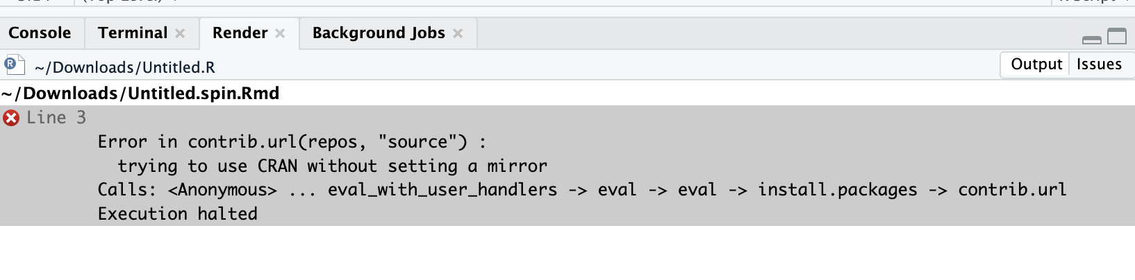
Installation of packages fails in scripts when you are trying to compile a report.
Image (CC0) by Kaidi Chen.Exactly the same syntax—install.packages("praise")—is
also used for re-installing it. You may want to re-install it if a
newer version comes out, of if you upgrade your R and receive warnings
about the package being built under a previous version of R.
After installation, the easiest way to get access to the provided
functions is by
loading the package with library() command:
## Load the package--
## make 'praise'-package functions available in this R session
library(praise)
Depending on the package and your setup, you may see various messages popping up on your console. These are typically harmless. But always pay some attention what is there, sometimes the messages may indicate problems.
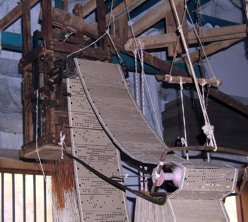
Jacquard loom in Varanasi, 2009. The chain of the control punch cards is clearly visible.
Steve.kimberley, CC BY-SA 3.0, via Wikimedia Commons
The word “library” denoting such collections of functions pre-dates computers. In early 1800-s, Joseph-Marie Jacquard invented semi-automatic loom to wave patterned silk fabrics. The patterns were stored on punch-cards, attached together to form a long chain. Each chain of cards represented a particular pattern, and these were stored in “libraries” of the patterns. A computing pioneer, Charles Babbage, borrowed the idea to use punch cards for computing, together with the word “library”.19
The other terminology he invented, “mill” for the processor and “store” for memory, did not stick.
library(praise)
makes the functions in the praise package available for R
(see more in the
documentation
for the description of the functionality of praise library). It
contains a fun function praise() that can praise you and your work!
For instance, if you think you personally need a boost, you can write:
## [1] "I am so luminous today!"This function, praise(), is not part of the core-R, but is located
in the library that we just loaded. Essentially R loaded a dedicated
script that provides this function (and more).
Do not forget to load the package with library() command. Unlike
installation, loading is needed to be done again every time you
restart R. And unlike installation, loading is fast and harmless. It
is well suited to use library() commands in scripts.
- adjective: words and phrases
- adverb
- adverb_manner: adverbs of manner
- created: synonyms of “create” in paste tense.
- creating: synonyms of “create” in present participle form.
- exclamation: positive exclamations
So if you need even more boost, you can write:
## [1] "Hurrah! You devised such a badass script!"Loading packages with library() command
is an easy and popular approach. However, what happens if more than one package call a function by the same name? For
instance, many packages implement function filter(). In this case
the more recent package will mask the function as defined by the
previous package. You will also see related warnings when you load the
library. In case you want to use a masked
function you can write something like package::function() in order to
call it. For instance, we can give you some extra praise with
## [1] "You are so LAUDABLE :-)"This approach—specifying namespace in front of the
function—ensures we access the function in the right package. If
we call all functions in this way, we don’t even have to load the
package with library() command. This is the preferred approach if you
only need to call functions of a large library for just a few times.
5.7 Writing Functions
Now when you are familiar with how to use the other peoples’ functions, it is time to write your own. Any time you have a task that you may repeat throughout a script—or sometimes when you just want to organize your code better—it’s a good practice to write a function to perform that task. This will limit repetition and reduce the likelihood of errors, as well as make things easier to read and understand (and thus identify flaws in your analysis).
Functions are in many ways just a few lines of “canned” code. Exactly as numbers and strings, they are normally stored in the “labeled boxes in memory”–assigned to variables.
5.7.1 Basics of defining functions
Let’s explain how to write functions through an example. We create a
function fullName that takes first name and last name as strings, and returns
full name, i.e. a single string made of the these names.
This is not particularly interesting function–it just concatenates two strings–but it helps us to explain all the major building blocks of functions.
Function definition contains several important pieces:
We assign the function to a variable (here
fullName). As in case of other variables, this means we store this chunk of code into memory, and label that memory area fullName.but what we store into memory is not numbers or characters, but R code. This code is put into a function using the syntax
function(....)to indicate that you are creating a function (and not a number or character string).the rest of the code follows the
function(...)declaration inside curly braces{ ... }.We often want to feed the function with certain inputs, here the first and last name. These inputs must be referred to somehow inside of your function. You list these in the parentheses in the
function(....)declaration. These are called formal arguments. Formal arguments will contain the actual values when calling the function (called actual arguments). For example, when we callfullName("Alice", "Kim"), the value of the first actual argument ("Alice") will be assigned to the first formal argument (first), and the value of the second actual argument ("Kim") will be assigned to the second formal argument (last). Inside the function’s body, both of these formal arguments behave exactly as ordinary variables with values “Alice” and “Kim” respectively.We could have made the formal argument names anything we wanted (
name_first,xyz, etc.). This is all well, as long as we also use the same names in the lines of code that makes the function body.The formal argument names are only valid within the function’s body (inside of the curly braces). Variables
first,last, andfullonly exist within this particular function. They are “forgotten” as soon as the function is done its job. If you try to access those outside of the function, you get and error likeError: object 'first' not found.Body: The body of the function is a block of code between curly braces
{ }(a “block” is represented by curly braces surrounding code statements). The opening brace{must follow thefunction(....)declaration, the closing}will complete the function–whatever follows the closing brace is not part of the function any more. The opening{is often put immediately after the arguments list, and the closing}on its own line.The function body specifies all the instructions (lines of code) that your function will perform. A function can contain as many lines of code as you want—you’ll usually want more than 1 to make it worth writing, but if you have more than fits to your screen, then you might want to break it up into separate functions. You can use the formal arguments here exactly as you use any other variables. You can also create new variables, call other functions, you can even declare functions inside functions… basically any code that you would write outside of a function can be written inside as well! One very useful trick is to print the values of local variables–this helps you to understand what is going on inside the function and spot the problems.
But remember that all the variables you create in the function body are local variables. These are only visible from within the function and “will be forgotten” as soon as the function is done–when you return from the function. However, variables defined outside of the function are visible from within too.
Return value is what your function produces. You can specify this by calling the
return()function and passing it the value that you wish your function to return. It is typically the last line of the function. Note that even though we returned a variable calledfull, that variable was local to the function and so doesn’t exist outside of it; thus we have to store the returned value into another variable if we want to use it later (for instance, asname <- fullName("Alice", "Kim")).
After we have defined the function, we can call (execute) it. We call a function we defined exactly in the same way we call built-in functions. For instance, we may call it as
## [1] "Alice Kim"When we do so, R will take the actual
arguments (here "Alice" and "Kim") and assign these to
the formal arguments (here first and last).
Then it executes each line of code in the
function body one at a time. Here the body only contains a single
line, paste(first, last), and when the actual arguments are
substituted in place of formal arguments,
it becomes paste("Alice", "Kim"). This, in turn produces "Alice Kim".
When it gets to the return() call, it
will end the function and return the given value. We can either
assign it to a variable, or print it right away as above.
Example 5.2 Let’s create a function that converts length given in feet to meters:
Now we can compute
## [1] 152.4i.e. elevation gain of 500ft on a trail is the same as having to climb 152.4 meters.

The supermassive black hole in M87 galaxy in polarized light.
Event Horizon Telescope, CC BY
4.0, via Wikimedia
Commons.
Exercise 5.12 The supermassive black hole in M87 is 55 millions of light-years
away.
Create a function ly2km that converts light-years to kilometers.
Use this function to compute distance to to the black hole in
kilometers.
See the solution
5.7.2 More details about functions
Now when you are familiar with the basics of functions, we discuss a few more easy and widely used details.
5.7.2.1 Return statement is optional
return() statement is usually not necessary in R as R implicitly returns
the last value it computes (last expression it evaluated)
anyway.20 So we may shorten the
definition fullName() function into
or even not store the concatenated names into full:
The last evaluation was concatenating the first and last name, and hence the full name will be automatically returned.
Example 5.3 The feet2m() function we created above can be writtng
in a shorter form as
This is exactly equivalent to the definition above, which one do you prefer is the question of coding style.
Exercise 5.13 Write a function decade()
that converts years to decade. Do not use
return statement.
Here is an example of a few years and the corresponding decades:
| year | decade |
|---|---|
| 2024 | 2020 |
| 1931 | 1930 |
| 1969 | 1960 |
| 1970 | 1970 |
Show that it works when you pass it these years.
Hint: use integer division %/%, see Section
4.4.1.
See the solution
5.7.3 Default argument values
Consider the fullName() function again. Now assume we have a lot of
peole who’s family name is “Kim”. We can get their full names as
## [1] "Alice Kim"## [1] "Eun-Gyeong Kim"## [1] "Ji-Won Kim"and so on. In that case we may want to write the function slightly
differently. We can make family name optional–if we do not supply
it, the function will take “Kim”, but if we want another names besides
“Kim”, we can supply it. This can be achieved through default
argument value in the form last = "Kim":
Now we can write
## [1] "Eun-Gyeong Kim"## [1] "Mongkut Sisuk"As you see, can use default values to make the code somewhat simpler.
In this example, the default argument is not very valuable: it is easy
to just write “Kim” as needed. But default arguments are widely used
in a different context–for functions that take a large number of
arguments. Imagine a function plot(). This might take a large
number of arguments: what to plot, how big the plot should be, which
color to use, whether to save it to a file, what should be the file
format… It is just too much work to supply all these arguments if
you just want to make a quick plot. This is where the defaults
help–the default arguments ensure you get a nice plot, and if you are
not happy with what you get, you can adjust it by changing some of the
default values.
Exercise 5.14 Write a function date() that takes 3 arguments: day, month, and
year, and returns the date as yyyy-mm-dd. If year is not
submitted, it will assume it is 2025. It should work like this:
See the solution
5.7.4 Returning values versus producing output
Unfortunately, the difference between functions that produce output (i.e. print on screen, see more in Producing output) and that return a value (that will be automatically printed on screen) may be less than obvious. For instance, consider two functions that compute minutes in day:
minutesDay1 <- function() {
   mid <- 24*60
   cat(mid, "\n")  # print the numbers
}
minutesDay2 <- function() {
   mid <- 24*60
   return(mid)  # return the number
}
When we call the former function on console, we get
## 1440and when we call the latter, we get
## [1] 1440The output produced by both functions appears almost the same. However, behind the scene (well, behind the screen 😄) there are important differences:
- The first function produces output, i.e. it always prints the
number 1440. The second function does not print anything. The
line
[1] 1440we see when we callminutesDay2(), that line is created by R console that automatically prints the last result. So in the second case1440is not something that the function prints, but the result, the return value that the R Console prints. - The difference may not matter when we run it like in the example above. But if we want to assign the result to a variable, then what happens is not the same any more:
## 1440minutesDay1() still prints 1440 but minutesDay2() is now
silent. This is because the result is not
automatically printed if it is assigned to a variable.
- The second function returns the value that can be assigned to a
variable (
mid2in this example). The first function automatically returns whatever its last statement,cat(mid, "\n")returns.
This happens to be the special empty symbolNULL:
## NULL## [1] 1440We can see mid1 variable is empty while mid2 contains the
expected value.
So the first example prints the result but does not return it, and the second function does not print it but returns the value. One can also create a function that does both (or neither). But which approach is better?
Obviously, it depends on what you are doing. In practice, it is common to have two types of functions–one type only prints and does not compute anything, and the other type only computes and returns a value, but leaves printing to the dedicated output functions.
Exercise 5.15 Create a function that takes a single argument, name, and returns a string: “Hi <name>, isn’t it a nice day today?” where <name> should be replaced by the argument name.
Demonstrate that the function prints the message when called on R console, but does not print anything if its result is assigned to a variable.
Hint: check out paste() and paste0() functions to concatenate strings.
See the solution
Exercise 5.16 Make a function that prints asivärk (see Section #ref()) and does not return anything (i.e. returns NULL). The function should have two arguments: number of lines to print, and the character to use.
Ensure it prints, even if the result is assigned to a variable; and that the variable remains empty.
The output might look like:
## ^
## ^^
## ^^^
## ^^^^
## NULL## 猫
## 猫猫
## 猫猫猫
## 猫猫猫猫
## 猫猫猫猫猫
## 猫猫猫猫猫猫
## 猫猫猫猫猫猫猫## NULLJames Essinger Jacquard’s Web: how a hand loom led to the birth of the information age, Oxford University Press, p 228.↩︎
When using RStudio, one can also load packages on the packages’ pane by clicking the respective checkboxes. There is also an install button for package installation. However, the former actually runs the
library()command and the laterinstall.packages()command. You will see these commands on console when you click the buttons there.↩︎Based on James Essinger Jacquard’s Web: how a hand loom led to the birth of the information age.↩︎
It is, however, necessary in certain other languages.↩︎