Chapter 3 What is data?
This section discusses the concept of data, what it is, how to handle it, and what issues are there you should be aware of.
3.1 What is data
3.1.1 Data and information
One of the central concepts in data sciene is data. It is in some ways the same as information, but in other ways not.
Data is often defined through information:Data is raw unprocessed facts and figures (raw information)
Information is processed data, ready to be used for understanding or decision-making.
| platform | timestamp |
|---|---|
| Windows | 2025-09-25 14:05:31 |
| Mac | 2025-09-25 14:05:32 |
| Mac | 2025-09-25 14:05:35 |
| Windows | 2025-09-25 14:05:37 |
| Mac | 2025-09-25 14:05:34 |
| Windows | 2025-09-25 14:05:36 |
| … | … |
For instance, the data about the platform students are using in this class might look in the table here. This is unprocessed raw facts, telling that Sept 25th at 2:05:31 a student claimed they are using Windows, a second later someone claimed they are using Mac, and so on. What can we use these data for?
| platform | N |
|---|---|
| Mac | 68 |
| Windows | 40 |
| Linux | 1 |
For instance, we may be interested in what kind of system support do we need in class. An obvious way to answer this question is just to count the Mac/Windows votes. We’ll end up with the table here.
This is processed data, distilled into information we can use in order to make decisions about the type of support that is needed.
Below, we consider data mainly as raw information, “facts and figures”, that is collected about some kind of particular objects.
Exercise 3.1 What kind of data might we collect about students in this class?
What kind of stories (conclusions) might we draw from these data?
How much can we trust these stories (conclusions)?
See the solution
But why do we want to have and use data in the first place? This is because we want our decisions to be based on evidence, on how the world actually works. And we can learn a lot about it from data–after all, data are a reflection of how the world works. So in a way, it is impossible to make informed decisions without data.
Now someone may claim that this is actually not true–for instance, we can do engineering calculations without any data, using just theoretical considerations. Yes, this is true. But how did we figure out the theoretical models that are the basis of such calculations? In fact, the theories were established and tested through data.4 So if an engineer designs a house using just her computer, without looking at any data at all, then all the data work was actually done long time ago and we already know the properties of the materials that are needed for the construction.
In practice, we often work the other way around: first we get data, and then we start looking what interesting things might these data tell. In a sense it is like a solution looking for a problem. But sometimes we can find an important problem where the solution fits.
Exercise 3.2
Consider two questions:- do students like pineapple on pizza?
- is pineapple a good pizza topping?
Can you answer these questions based on data? How would the dataset look like?
See the solution
See Section 3.3 below for more discussion about data and information.
3.2 Different kinds of data
TBD: move behind Data and Information; merge the latter with What is Data
Through this course we mainly consider data in electronic form, in a form that is suitable for computers. But data can be in many different forms and types.
Most of data we discuss in this book is a table of numbers in electronic form (see more about data frames in Section 3.6), but data may also be in a very different format. For instance an image, a printed book, or an oral tradition can all called “data”.
3.2.1 Numeric data
One of the most common data types, and one that is easy to handle, is numeric data. There are many things that are measured in numbers, and numbers are easy to analyze mathematically. We can also compute figures, such as mean and minimum value. Numbers can also be easily compared.
Below is an example of small set of numeric data, length of iris setosa flower sepals (leafs) in cm (see more in Section B.6):
## 6.3, 4.9, 5, 5, 6, 5.7This displays lengths of six sepals. We can also make various useful calculations, e.g. find the mean length (it is 5.48 cm), and we can tell that the first flower in this sample has longer sepals that the last one.
Numeric data is usually displayed in obvious form, such as “2” or “-3.14”. If numbers are very large or very small, they are displayed in exponential form. For instance,
## [1] 2.4e+10## [1] 4.166667e-11The former must be read as \(2.4 \cdot 10^{10}\)
and the latter as \(4.166667\cdot 10^{-11}\). So e+ or e- in the middle of the number means the
powers of ten.
3.2.2 Categorical Data
Another widely used type of data is categorical data. For instance, data about college majors may look like
## Real Estate
## Pre Social Sciences
## Arts and Sciences
## Psychology
## Arts and Sciences
## Chemistry
Categories are often coded as text, but they are, strictly speaking, not the same as text data (see Section 3.2.3). Categorical data is categorical if there is only a limited number of valid categories.
We can do various interesting computations with categorical data, but some of what is possible with numbers may not be possible with categorical values. For instance, we cannot compute “mean major”, and we cannot tell if the first major (Real Estate) is larger or smaller than the last one (Chemistry). These questions just do not make sense. But we can compute the frequency (count) of each major, here we have Arts and Sciences represented twice, and all other majors a single time.
Sometimes the categories have an inherent ordering. For instance, consider the categories “strongly against”, “somewhat against”, “indifferent”, “somewhat supportive”, “strongly supportive”. Although we cannot tell whether one is larger than the other, we can say that “somewhat supportive” is more supportive that “somewhat against”. Such ordered categories are widely used in opinion surveys (and called “Likert scale”). They are frequently coded as numbers (e.g. “strongly against”=1, …, “strongly supportive”=5), but this is deception. These are not actually numbers, even if coded so. This is because you cannot make any meaningful mathematics with such values.
Exercise 3.3 Find data that contains such ordered values. How is it coded?
3.2.3 Text data
Text data is somewhat similar to categorical data in a sense that its values are textual, not numeric. But unlike categorical data, text data does not have to fit into any pre-defined category. For instance, tweets or user reviews are text data, but the name of your favorite color is not. The former have no limit in terms of what they contain (there are typically length limits though), but the color name must be a real color name.
We do not discuss text data in this course.
3.2.4 Other data types
There are a plethora of other data types. Some numerical data can only contain certain kind of values. For instance, number of children in household must be a non-negative integer. A separate and surprisingly complex data type is date and time. It turns out that it is not trivial to describe date and time in a coherent way that allows for different time zones, time intervals, consistent handling of both dates and times, and so on.
Another large class of data is image and audio data. Although these can and are stored numerically, this is not the way we usually experience these data. They also tend to require noticeable more memory and processing power. In this course we do not work with images and audio.
Finally, data does not have to be in electronic form. Old receipts, printed books, photos on paper, vinyl LP-s and oral traditions, all contain similar data–just not in a form that is ready to be analyzed on computer. But nevertheless, it is data!
3.3 Data and information
When think about data and data processing, then usually what we care about at the end is neither data nor the process. We care about some sort of result, an answer to a question we are interested in. And data only matters as far as it helps to answer that question. We may have an enormous amount of data but still not be able to answer the question. In this sense it may be helpful to distinguish between data — the amount of numbers, categories, variables and records do we have —, and information — how well can we answer our question based on data. Such definitions of data and information is useful, but not universal.
As an example, consider the following. We notice that every morning the rooster crows and a few minutes later the sun rises. Did the rooster’s crow made the sun to rise? Was the sun waiting for the “go ahead” by the rooster? What kind of data we need to figure this out? Say we collect data about timing of the crow and sunrise. We may see a dataset that looks like
| Date | First Crow | Sunrise |
|---|---|---|
| 2022-09-23 | 6:45 | 6:50 |
| 2022-09-24 | 6:46 | 6:51 |
| 2022-09-25 | 6:47 | 6:52 |
| 2022-09-26 | 6:48 | 6:53 |
| 2022-09-27 | 6:49 | 6:54 |
| 2022-09-28 | 6:50 | 6:55 |
These data do not tell us if the sun was waiting for rooster’s “signal”, or rooster just started crowing a few minutes before the sunrise because the sky was becoming bright. (Well, we know that the second explanation is correct but our knowledge is not based on these data!) Crucially, the problem is not in the amount of data–if we were to collect similar data for more weeks, months or years, we still weren’t able to answer the question. Even billions of records would not help. The dataset just does not contain the information that is needed to answer the question.
Exercise 3.4 What kind of features should the dataset contain for us being able to tell if sun is waiting for the rooster or the way around?
See the solution
A crucial point in understanding what can be done with a dataset is to know what is not in data. Imagine you want to know if students like pineapple on pizza. What might be easier than to go to a pizza place and ask all students there?
But this approach misses a crucial part of students–those who do not go to the pizza place. Even more, the reason they do not go there may be that they do not like pizza, neither with pineapple nor without it. Unless we know that those students were excluded, we cannot even tell what can be done with these dataset. We need to know how the data were collected!
But note that even if we know that, if we learned that the information was just collected by someone who was asking students at the pizza line, we may not be able to tell if adding more (or fewer) options with pineapple is a good idea. Maybe we should offer more fried rice dishes instead? These data are not enough to tell.
Exercise 3.5 You want to prove, based on data, that all ravens are black. How would the relevant dataset look like? Can you, in principle, prove this claim if you could collect suitable data?
See the solution
Typically, we gain invaluable knowledge about the dataset from its documentation. At least some documentation is almost always needed, at least we should understand the basic facts like what is this dataset about; what are the most important variables there; and how is the sample selected. Good documentation covers all this in-depth, and also includes other fact, e.g. who funded data collection, what are the usage rights, and more.
Unfortunately, good documentation is scarce. This is partly because it is a lot of work to compile documentation, partly because certain tasks require less than others, and partly because lack of documentation may avoid certain privacy-related questions. But for the data user, it may mean that we have to do a lot of guesswork, or that we cannot use it for our purpose at all.
Example 3.1 Heart attack dataset (See Section B.4) contains information about medical symptoms and whether the patient had a heart attack. It originates from kaggle, and you can also find some documentation there. An example of the dataset looks like:
| age | output | sex | cp | trtbps | chol | restecg | oldpeak |
|---|---|---|---|---|---|---|---|
| 61 | 0 | 1 | 0 | 140 | 207 | 0 | 1.9 |
| 55 | 0 | 0 | 0 | 180 | 327 | 2 | 3.4 |
| 34 | 1 | 0 | 1 | 118 | 210 | 1 | 0.7 |
| 48 | 0 | 1 | 1 | 110 | 229 | 1 | 1.0 |
| 51 | 1 | 1 | 2 | 100 | 222 | 1 | 1.2 |
The data source includes documentation of the variables (see Section B.4). For instance, we learn that cp (chest pain) can have four distinct values: 1–typical angina; 2–atypical angina; 3–non-anginal pain; 4-asymptomatic. However, a brief look at the table above (column 4) indicates that cp can also have value “0”. Hence data and documentation do not match completely.
3.4 Data integrity: How is data collected?
Not all kinds of data can be used to draw meaningful conclusions. Even more, in order to use the results for serious conclusions, the data must be collected in a very specific way, and the related procedures must be clearly documented. Collected data also needs validation, checking that it actually was collected in the way we intended.
Trustworthy data collection typically includes the following steps:
- what is the relevant population? If we intend to collect data about voters, do we intend to represent all eligible voters? Only voters in certain segment? Maybe only those voters that are likely to actually vote?
- Sampling: How is data collected? Sample is the subset of the population that we end up getting our data about. Even if we intended to cover all voters, but ended up only talking to a few friends, the dataset is probably not going to tell much about the electorate as a whole. We need to take steps to ensure that it actually represents the relevant population.
- Who collected data? We would prefer it to be a neutral institution that does not want to prove that one or another political party has more support.
- Coding: how are the values coded? In some cases it is simple, e.g. age is typically coded in years. But what might be income values “1”, “2”, “3” and “9”? Or political preferences “-1”, “0”, “1” and “5”? Unless we have credible documentation, we cannot really tell what these values are.
- Where did you get the data? Even if the original dataset was collected in a trustworthy manner, there may be various problematic copies around.
Exercise 3.6 I want to know what percentage of students lives off campus. As I am lazy, I just ask this question from students in my class.
- What is the population?
- What is the sample?
- Do you think the sampling scheme is trustworthy? Why?
Unfortunately, collecting a good reliable dataset about human subjects is a major work. Analyzing humans is further complicated by the privacy issues—in most cases the data is not made easily available for the interested parts, e.g. for college students. On the other hand, many big corporations, such as cellphone providers, collect a lot of individual data, but as the sampling procedures are not known, these cannot be easily used for analysis.
Even if the analysis that is done based on non-trustworthy data is correct from the statistical point of view, the problematic data makes it dubious. Carbage in–carbage out.
Example 3.2 Let’s return to the heart attack data. Above, we discussed that certain variables are not documented.
But even worse, the documentation is silent about how and where is the data collected. Is it a sample of general population? Is it a sample of patients, hospitalized with suspected heart attack? We do not know. And hence we cannot use these data for any medical analysis.
3.5 Data storage, privacy, ethics
The technical side of data storage is relatively straightforward. It is normally stored in computer hard disks, or maybe in archives if it is on paper. Your personal computer probably contains various amounts of data, including your photos, your chat logs and similar, you also have a number of printed books and pictures at home.
However, if one wants to store data for extended period of time (more than typical lifetime of a laptop, about 5 years), then more serious arrangements are needed. These are less technical on more organizational. After all, most common electronic data storage methods cannot are not reliable for more than a few years, so one needs to make regular backups, ensure the backups are error-free, and replace the storage medium from time to time. This is an important task for large and valuable datasets, such as government health data, or bank’s transaction records.
Next to data storage, there is the question of ownership. As data is inherently non-rival good,5 the ownership is murky to begin with. Often data ownership is claimed by the institutions who published the cleaned dataset that may originate from various sources. Sometimes users have either to sign non-disclosuer agreements, or to pay to these institutions in order to use data. But in recent years a different ownership ideas have been voiced more often, namely that the original data sources (for instance the individuals whose data is collected) should have a share in the ownership. Such ideas are still in early stages, but it is hard to believe the powerful institutions are going to share much of their wealth and power with dilute data sources.
Often data owners are also gatekeepers who can decide who can access data, and under which circumstances. Many of public owners publish a lot of data on internet for everyone to use without any extra requirements. For instance, City of Seattle puts a number of interesting datasets up at the Seattle Open Data page data.seattle.gov. This includes data about street life, criminal incidents and public sector salaries.
But not all kinds of data can be freely published by the owner. Most of data about humans, such as their income, health, education records and so one, are legally protected in one form or another in most jurisdictions. So even if you are a doctor who has examined a number of patients and in this way “own” the corresponding data, you cannot just publish it on internet. Such data is normally only available for established research or government institutions under strict non-disclosure and data security agreements.
Exercise 3.7 Universities collect a lot of data about students through the way the function. This includes everything about the classes students take and grades they get, but various additional information, such as health and membership in student organizations. in the U.S. universities, these data must be stored and handled in FERPA compliant way.
What is FERPA and how does it require to handle the educational data?
As data is a valuable resource, possessing data also gives one power. While this sounds like a nice thing to have, most of us are not ready for the related security risks. In the developed part of the world, security often means some shady hackers stealing data from your computer. However in the less stable environment it may also mean gunmen who bang on your door and ask for your laptop and passwords. Or maybe you will be subject to a brutal interrogation, because you are using “wrong” data, at least according to the authoritarian government. So in an uncertain environment, the best choice may actually be not to just delete data as soon as possible, or not to collect these in the first place.
Unfortunately, the privacy and security concerns make original research, and replication of other results, much more complicated. For instance, there are very few datasets that contain individual income and health data that can be used in teaching. There is a large number of various income and health datasets and many advanced economies offer options for various kinds of cross-links of education, health, income, tax records and such information. But in order to get access to such datasets one needs to be a member of an academic or another comparable research institution, submit a lengthy project description, and get the necessary approvals.
3.6 Data frame
Data, when already in electronic form, may come in various formats. It may be just a list of numbers (like the iris sepal length data above) or categories (like the list of college majors). But quite often we encounter data where many related values are grouped together, and we see a number of similar groups. This is the essence of data frame.
3.6.1 Data frame–a table of rows and columns
You have already seen a few examples of data frames. The sunrise data above was one: date, crowing time and sunrise time are grouped together (we can call that group a daily observation). And six such groups are placed underneath each other.
Here is another sample data frame, describing the passengers of the ocean liner Titanic that sank in 1912:
| name | age | survived | pclass | sex | fare |
|---|---|---|---|---|---|
| Richards, Master. George Sibley | 0.8333 | 1 | 2 | male | 18.7500 |
| Ashby, Mr. John | 57.0000 | 0 | 2 | male | 13.0000 |
| Parr, Mr. William Henry Marsh | NA | 0 | 1 | male | 0.0000 |
| Richards, Mrs. Sidney (Emily Hocking) | 24.0000 | 1 | 2 | female | 18.7500 |
| O’Leary, Miss. Hanora “Norah” | NA | 1 | 3 | female | 7.8292 |
| Beavan, Mr. William Thomas | 19.0000 | 0 | 3 | male | 8.0500 |
In this example, each row represents a Titanic passenger. The table displays six pieces of information about each passenger. These are name (passenger’s name); survived, whether they survived (1) or not (0) the shipwreck; pclass tells which passenger class did they travel (1, 2, and 3), sex is either male or female, and fare is fare paid (in UK pounds of 1912). For instance, the first record in this example is about Master. George S. Richards, a 10 month old boy, who traveled in second class and survived. His fare was 18.75 pounds.
Data frames are typically displayed as similar rectangular tables. Rows are often called observations, but also cases or just rows. Columns in such a table displays different features. The columns are called variables, but you may also see features, attributes, or just columns.
It is crucial to understand what do the rows represent when working with data frames. In the Titanic example they represent different passengers, and in the rooster example they represent different days. But sometimes the meaning of a row may be more complex. For instance, here is a snippet of Scandinavian COVID-19 data:
| country | date | type | count | population |
|---|---|---|---|---|
| Finland | 2020-08-14 | Confirmed | 7700 | 5528737 |
| Finland | 2020-08-14 | Deaths | 333 | 5528737 |
| Finland | 2020-08-15 | Confirmed | 7720 | 5528737 |
| Finland | 2020-08-15 | Deaths | 333 | 5528737 |
| Finland | 2020-08-16 | Confirmed | 7731 | 5528737 |
| Finland | 2020-08-16 | Deaths | 333 | 5528737 |
What does an observation represent here? It cannot be a country because all these rows are about Finland. It cannot be a day, because there are two rows for each day. It also cannot be type, because there are multiple rows with Deaths and Confirmed. In fact, each row here represents a unique country-date-type combination. So the first row tells how many confirmed COVID-19 cases there was in Finland on August 14th, 2020, and the following one tells how many COVID-19 deaths there was in the same country for the same date. (There are also similar rows for other countries).
Exercise 3.8 Write down your name and favorite color. You have created a tiny data frame.
- What are the variables (columns)?
- What might the rows represent?
See the solution
Exercise 3.9 Consider a dataset about students’ grades.
- What might be the variables?
- What might the observations represent?
- Sketch a few columns and rows of such a data frame.
See the solution
Exercise 3.10 Why is name text and not categorical?
See the solution
pclass is a bit tricky variable: it is coded as a number (“1” for the 1st class, 2 for 2nd and so on). But these numbers are actually not numbers: you cannot do any regular math with these numbers—we cannot say that 1st class plus 2nd class equals 3rd class. These are just categories, but coded as numbers. So pclass is a categorical variable—you may as well replace the numbers with words like “first” and “second”.
Finally, survived is categorical as well as we cannot add or multiply life and death in any meaningful fashion. However, such two-category variables (typically called dummies), can often be treated as numbers from the technical perspective.
Such a quick look at the data frame also tells us something about the data quality. Most of the values look reasonable. It is perfectly feasible that a 10-month old baby George survived, and 57-old John Asby died. But in the third row we see some weird results. First, Mr William H. M. Parr’s age is given as “NA”. This stands for “not available”, and probably means the data creators (the investigation committee) did not know how old was this passenger. Obviously, there may be other reasons, for instance they just forgot to fill in his age. We also see that he paid 0 pounds for his first class ticket. It is technically possible, but again, it is very suspicious. It is more likely that the data compilers did not know fare paid, and just wrote “0” in that place. Or maybe a missing value marker was replaced by “0” by certain software before the final data file got to our computers. We just do not know. But overall, as the example table only contains two problematic entries (there is another missing age), it suggests that the dataset is of reasonably good quality.
3.6.2 CSV-files
In this course we focus on CSV files as our main data source. CSV stands for Comma Separated Variables, and it is a very popular way to store various types of data. In essence, it is just a text file that contains a data frame. Each row in the file represents one row in the data frame. Commas or other symbols split the rows into columns. For instance, in the figure below, the first rows contains columns pclass, survived and name. These are column names, csv files typically contain column names (but this is not always true).
The figure below shows an excerpt from Titanic data as csv file, separated by commas (left) and tab-symbols (right).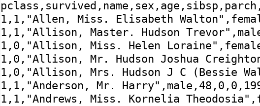
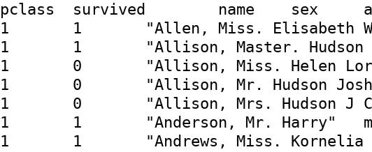
Two examples of CSV files. The left side of the image shows a csv with commas as separators. It is a plain text where there are commas between different values on the same row. The right hand side shows the exact same dataset using tab as the separator. This version is somewhat easier to read for humans, but for computers, these two variants are equally good.
Obviously, one can use other characters instead of comma to separate the columns. On the right hand side of the figure the same data is displayed using tab as the separator. But even if using something else than comma, the files is still typically called “csv files”. As csv files are just plain text files, one can load one into a text editor, such as RStudio, and modify it. You can even create a new csv files from scratch in this way.
3.6.3 Data frames and data vectors
It is not always you need a table–the data frame. Sometimes a 1-dimensional sequence is good enough.
TBD: data vectors
3.6.4 Limitations of data frames
Data frames is a popular way to represent data, but not all data can be converted to data frames (and hence to csv files). This is because data frames are rectangular tables: every row has the same columns, and each column is present for every row (some values may be missing though).
But this is not a good way to store very heterogeneous data. If each row would have different variables (columns), then it is fairly worthless to squeeze it into a data frame.
Imagine data about industrial tests where each time we test a very different item. Some data may be common, such as time of the test and the tester’s name, but others may be completely different. When testing a battery, we want to record initial voltage and energy, discharge, temperature, leakage current and such parameters. When the next record contains test of wine glasses, then instead of voltages and currents, we may want to record color, clarity, and sound. We may also test whether the glass survives a drop. There are too little common values for it being worthwhile to combine these two tests into a single data frame.
TBD: real example
3.7 Loading and exploring data
There is a variety of ways to analyze data. Below, we are using R language in RStudio environment (see Section 2). There is a plethora of ways to use R, here we rely on tidyverse framework, a set of tools developed by Hadley Wickham to make R more accessible for those with minimal coding interests. We assume you have installed it, see Section 2.8.
As the first step, we load the tidyverse set of packages:
If all is well, it should print a number of messages but no errors.
In the example below, we load Titanic data. If you intend to follow these example, you can download it from that link. Store it into the folder where you run your RStudio, you may also create a separate folder for these examples.
Next, we will load the dataset. It can be loaded with a command
This should load the dataset, and give it a name–“titanic”. R can
hold multiple datasets in memory and we refer to those through their
names. So the command we did above actually contains two parts:
read_delim("titanic.csv") loads data, and titanic <- stores it
in memory under the name “titanic”. Note that the function we use
here is read_delim() (with underscore), there is also a function
read.delim (with dot). Here we consistently use the former,
read_delim(). These functions are fairly similar, just the
underscore–version can automatically guess the correct CSV file separator.
Note also that the file
name–titanic.csv– must be quoted.
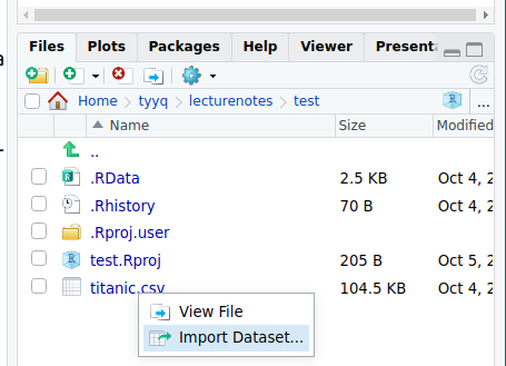
You can invoke the data importer through the Files tab in RStudio.
Alternatively, you can choose the R data importer to load the data file. This can be invoked from the Files tab (in the lower-right pane) by clicking on the data file name and selection “Import Dataset”.
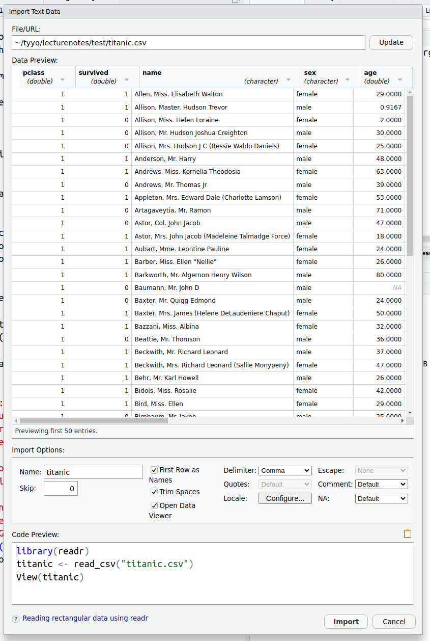
R data importer in action.
The data importer allows you to pick various options, in particular select the file separator and pick the name for the dataset in memory. You get some visual feedback to understand if the dataset will be loaded correctly. Underneath, you also see the corresponding R code–the data importer does not just import data, but creates a short script that loads data. If you wish, you can copy the code to your script window and amend it for your own purpose.
In this example, the last command, View(titanic), will open the
dataset in the data viewer.
Exercise 3.11 Choose to open the Titanic dataset in the data importer. But now pick a different separator (Delimiter) instead of “Comma”, e.g “Tab”.
- What happens to the code?
- What happens to data preview? Do you understand why?
See the solution
Here we chose to call the loaded data frame “titanic”. We do not have to call it like that, names like “t”, “Titanic”, or “x” are also perfectly good names. But when you have multiple data frames in memory then it may get too confusing. A good choice is to pick a word that describes the data well and is easy to remember.
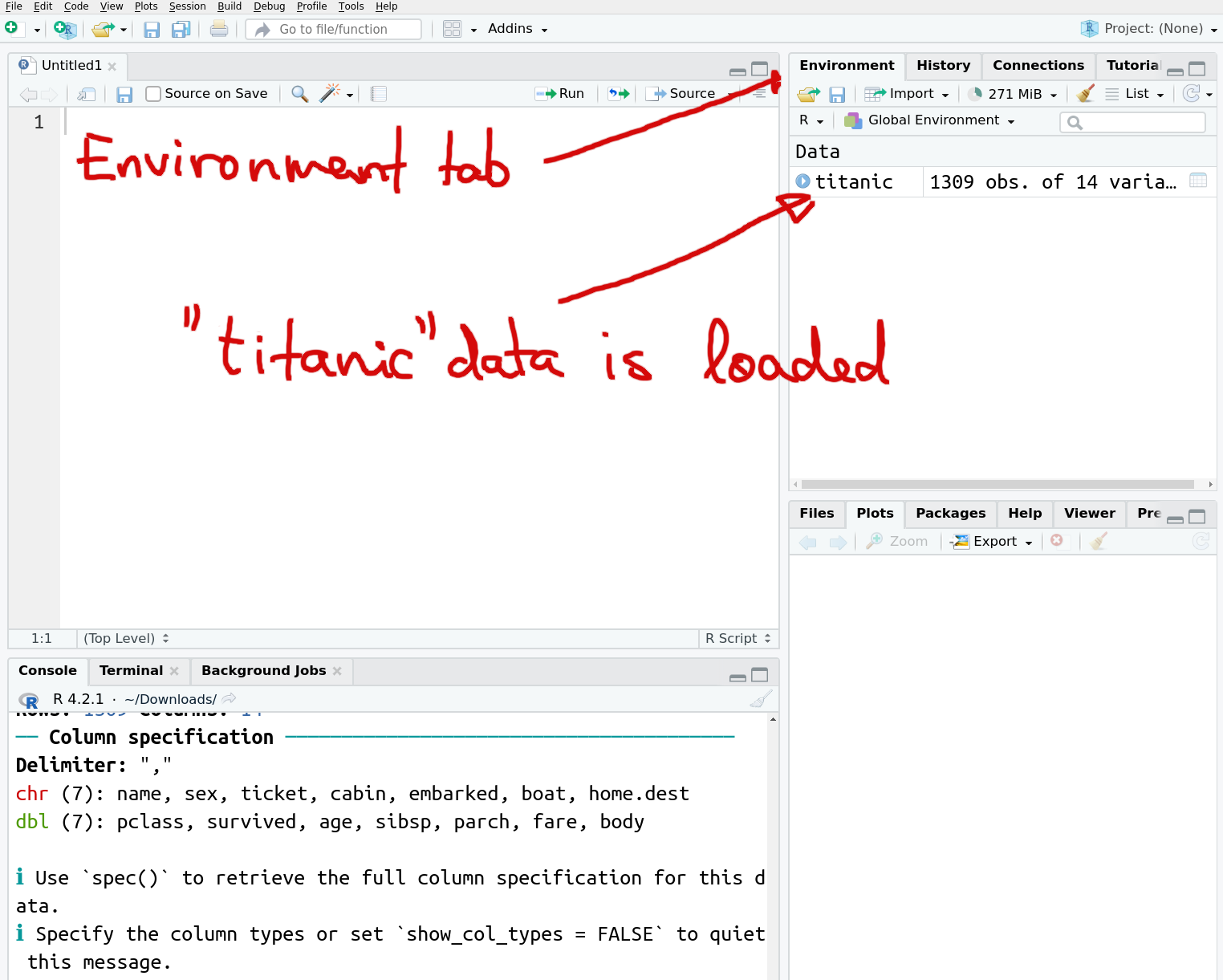
How RStudio looks after the dataset is loaded. The “Environment” tab shows a new dataset, “titanic”.
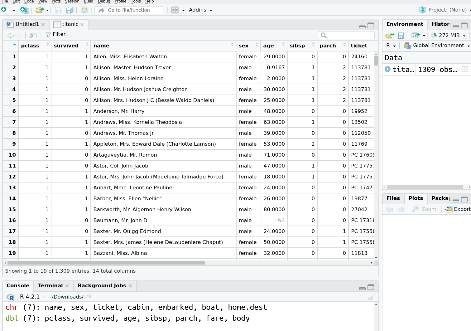
RStudio data viewer. The leftmost, light blue column is the row number, all other columns are data variables.
The data viewer let’s you, well, view your data. It displays the columns (variables) in data in bold, the leftmost (light blue) column is not a variable but a row number. We can see that all the first 19 passengers on this image were traveling in 1st class, there were survivors and victims, and men and women among them.
The data viewer also let’s you do do some simple analysis (commands are much more powerful analysis tools though). For instance, by clicking on columns, you can sort the dataset in one way or another.Exercise 3.12 Use the data viewer to find out how much did Daniel, Mr. Robert Williams pay for the trip? In which class did he travel? Did he survive?
Hint: order the passenger list by name, or use the search bar!
See the solution
We can also explore the other columns.
Exercise 3.13 Explore the variables boat and body. What do you think they mean? Why do the contain so many missings? Do you think it indicates that these data are problematic?
Next, let’s do some additional data manipulations using commands. Above (see Section 3.6) we noticed that at least one passenger did not pay any money for his first class ticket (or so the data seems to indicate). How many of such freeriders do we find in data?
This creates a new dataset, called freeriders in the environment. You can double-click on it to open it in the data viewer. But the anatomy of the command is as follows:
- Take titanic dataset (
titanic) - feed it into the
filterfunction (%>%) - filter, keep only rows, where fare is zero (
filter(fare == 0)) - store the result (only these rows into a new dataset freeriders
in memory (
freeriders <-).
Note the following:
- the composite command like here mostly follows a logical “recipe”: take titanic data, filter for rows where fare is zero.
- just the storing the result back to memory is done on the first row, as the first two elements.
- we refer to data frame columns (data variables) using their names
(note
fareinfilter). This is a general behavior of R (and other programming languages): data and variables are referred to using their names. - finally, equality is tested using double equal sign
==.
Next, we can take a look at the freeriders dataset in the data viewer. Note that while technically it is just a subset of titanic data, from R-s perspective, it is a completely different dataset with its own dedicated location in memory. If you modify, or even delete titanic, freeriders will not be affected in any way.
A quick look at freeriders dataset shows that there are 17 persons, all of them male. They were traveling in all passenger classes. Sadly, only two of them survived.
Exercise 3.14 Look at how many age values are missing in the freerider’s data, and compare this to the frequency of missing age values in titanic data. What do you think, what does it tell you about the quality of information we have (i.e. the investigation committee had) about these people?
3.8 What is data science
Data science is an interdisciplinary field that contains computing, statistics, and field knowledge. As other similar fields, there are many attempts to define it, and we will probably never get into a universally accepted definition. But a common definition contains three main branches:
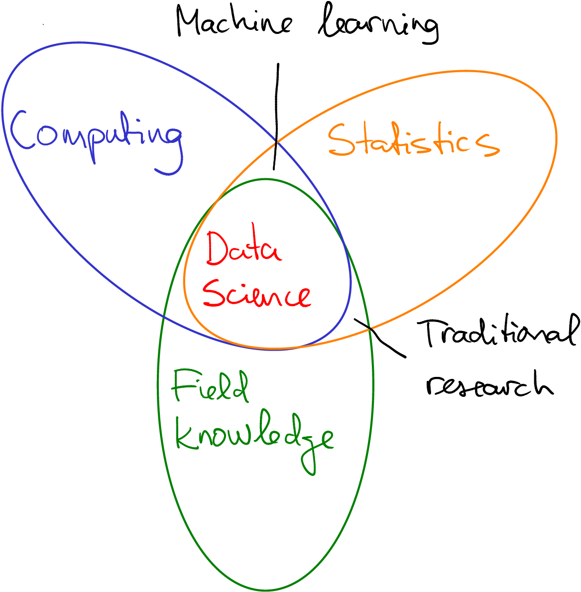
Data science can be understood as an intersection of computing, statistics and field knowledge.
- Computing. Data science is typically done using computers on large-ish datasets, and this requires good skills to use computers and the relevant software. Depending on the data used, processing it from its initial form to the form that can actually be used for answering the questions by be quite complex. Traditionally it is done using programming using languages and frameworks, such as R, python, OpenCL or spark. But one can do a lot with little to no coding experience. After all, one of the crucial tasks is to understand data and understand the questions you want to answer with the data. This can be done without coding.
- Statistics. After the initial data processing you need to answer your questions. This typically means using certain statistical methods. These can be as simple as a \(t\)-test, or as complex as neural networks. So data science employs a lot of statistics, some of it that is the traditional field of statisticians, some of it that is more commonly done by computer scientists. The statistician-self of data scientist should be able to choose a relevant method, and evaluate the goodness of your answer.
- Field knowledge. Finally, it is not enough the be able to process data and answer the questions. One should also be able to come up with relevant questions, and understand the answers. This requires you to know about the field. If we talk about education access for low socio-economic status groups, you should know something about education, about poverty, how these two are related, and what we already know about these problems. And when we get an answer from data, we should be able to evaluate its significance–is it something we already know? Is it plausible? Can it be used for some meaningful decisions?
In this sense, data science is nothing new. All these tasks have been around for decades, if not centuries. But as such combination of skills become more and more valuable in the 21st century, people started to call it “data science”. Obviously, one cannot be a top specialist in all these fields. You can easily do a PhD in computing, another in statistics, and a third in e.g. sociology. We have either to specialize, for instance you can be very good in your field much less good with computing and statistics, or you can also become a jack-of-all-trades but a master of none.
Data science has large overlaps with both computer science and statistics. But unlike data scientists, statisticians thend to focus more on statistical theory and methods, and less on particular compute-intensive applications and data management. Computer scientists, in turn, focus more on computing algorithms, but not that much about statistical methods or data ethics.
Data science has become common in fields where large and complex datasets are increasingly available. This includes e.g. satellite imagery, large telescopes, CERN, but also many large enterprises, such as Google or Amazon, that by their nature collect a lot of data. Before we can start using these data in statistical applications and decision making, we need to transform it into a more informative and more manageable form. This is a large part of work that data scientists do.
Typically, data scientists perform tasks that can also be done by someone in one of these fields. They locate and aquire data, describe and transform it, devise statistical models that target the problems under considerations, run these models and get answers, visualize the answers, and present and discuss the results. To do all this well requires a wide and diverse skillset.
The three big types of analyses usually done with data are
- exploration. This includes various “quick” look at data. What kind of information we have in data? Do we have information we are interested in? Can we compare, for instance, the average fare price of first class and third class passengers? This includes the examples we did above in Section 3.7, but exploratory analysis can also be much more complex (see below). Exploratory analysis is typically the first part of all sorts of analysis–before we can use data for any particular purpose, we have to understand it. And exploratory analysis is a perfect way to learn about your data.
- inference is using data to tell something about the world. Questions like “does the drug cure illness?”, “does the training program work?” and “is the global temperature in 2010-s higher than in 1980-s?” belong to this category. Note that inferential analysis provides answers about the world based on data, it is not the same as answering the same question about data. Inferential analysis is heavily relying on statistical methods.
- Finally, another common task is prediction. Instead of trying to tell something about the world, we are asking questions about a a particular person or date: will this patient heal if she takes the drug? Will that worker get a better job if he takes the training? Will it be raining tomorrow? We typically need some knowledge about “how the world works” before we can do predictions, but here we are not concerned about the world. We are interested in the particular cases only.
We talk about empirical sciences here. Whether mathematics is using “data” can be debated.↩︎
Non-rival goods are such goods that are not “used up” unlike traditional goods. If I eat a piece of cake, a traditional rival good, the you cannot eat it. But if I use data, a non-rival good, you can still use it.↩︎