Chapter 12 Statistical Inference
In Section 7 we introduced descriptive statistics. This section is devoted to inferential statistics–using statistical tools to say something about the “whole” based on a sample. As you can imagine, such task, using one thing (sample) to say something about another thing (the “whole”) is more complicated, and requires both more careful data collection and more complex analytical methods. This section is devoted on these tasks.
12.1 Population and sample
As we briefly discussed in Section 7, inferential statistics is concerned about telling something about the “whole” based on “sample”. For instance, if you are working for election polling, you may want to use your sample of voters (typically around 1000) to tell something about the election outcome (typically decided by millions of voters).
But before we start, let’s make clear what is the “whole” and what is the “sample”. In the most intuitive case, the “whole” is population, such as all voters in case of election forecasting. Sample, in turn is a small subset of the population, for instance a poll conducted among the voters. In national elections, millions of voters cast their ballots, while the forecasters typically work on a sample of 1000 voters only. Population is much much larger than the poll, in fact we typically think that the population is of infinite size.

Knucklebones, like this medieval bone from a shipwreck in Northern Europe, are a form of dice, used to play games. Unlike modern coins, they are likely not fair.
Rijksdienst voor het Cultureel Erfgoed, CC BY-SA 4.0, via Wikimedia Commons_van_rund_(bos)_-_O36ZFL_-_60015676_-_RCE.jpg)
But not all “populations” are like voters. For instance, you may try to determine if a coin is biased. You may flip the coin ten times and count heads and tails. This is the sample of size 10. But what is the “whole” or the “population” here? One can think in terms of all other similar coins out there, but actually this is not the case. After all, you flip just a single one, so the other similar coins do not play a role. Instead, you can imagine that the “whole” is all possible flips of the same coin. You can imagine that there is an infinite number of coin flips “out there”, and you just sampled 10 of those. The population–infinite number of flips–is not the flips, it is just a property of the coin. Either it is unbiased (it will tend to give 50% of one side and 50% of the other side when flipped), or it may be biased. So in this case “population” is not really a population but a property of a single object.25 But fortunately, we can analyze such properties of the coins in exactly the same way as we analyze voters.
Finally, there are examples where it is not possible to get a sample of more than one. For instance, what samply you might collect data to answer the question: “what is the chance that it will be raining tomorrow?” There will be one and only one tomorrow, and in that tomorrow it will either be raining or not. We cannot collect a sample of more than one tomorrows. Even more, if we want to answer this question today in order to decide about a picnic in a park, then we cannot collect even the sample of one. We can still think in terms of all possible tomorrows, but we have to answer it without any sample at all.
Below, we limit our discussion with the “voter example” where there exists a large population, population that is much larger than any sample we can realistically collect.
12.2 Different ways of sampling data
For many tasks it is extremely important to know what cases from the population end up in the sample. This process–what are the criteria that make certain cases to end up in the sample–is called sampling. There is a plethora of ways to make a sample, and frequently we do not know what exactly was the process. Here we discuss a few common ways to do sampling, and the problems related to different sampling methods.
12.2.1 Complete sample
complete sample is the case where we can actually measure every single subject of interest. For instance, we can sample every single student who takes the course. This is perhaps the simplest possible sampling method, in a sense it is not sampling at all but we are observing the population instead.
But complete sampling has a number of problems.
First, and most obviously, it may not be feasible to sample everyone. Think about the election polls where the pollsters should survey hundreds of millions of people. This is prohibitively expensive.

Fireworks are wonderful, but each rocket can only be used once. Hence you have to rely on a sample to test the products.
Seattle, July 4th 2022.Second, for many tasks, “sampling” also means destroying the object (called destructive testing). Imagine you are working in a factory that produces fireworks. You follow the specifications and the safety protocols–but do your rockets actually work as intended? The only way to find it out is to “go bang” and try them out! But you only want to do this with a small sample–complete sample would mean to shoot all your rockets and leave nothing to sell…
Third, even if you sampled everyone, are you sure that you actually observed everyone? This may sound like a semantic nitpicking, but it is actually an important question. The answer depends on what exactly do you want to do. If you are only interested in students in that particular class, in that particular quarter, taught by that particular professor, then observing everyone who takes the class is indeed a complete sample. But often we are interested in a more general question–for instance we want to know something about all students who take that class, including the past and future ones. Sampling everyone in the current quarter is not the complete sample any more.
This question is also discussed in Section 7.1.
Finally, quite often the problem is not that we cannot sample everyone, it may actually quite easy to take into account the resulting uncertainty. Instead, the problem is that we do not know who exactly ends up in our sample. This may result in biased data (see Section 12.2.4) and wrong results.
12.2.2 Random sample
The case where all subjects in the population have equal probability to end up in the sample is commonly called random sample.26 This is perhaps the simplest sample one can do, and it’s properties are well understood. Although it is simple, it may be hard to achieve, and in other cases it may not even be desirable.
An example of random sampling might be a household survey. Out of all households in a city, the survey may randomly select a smaller number (say, 1000). Nowadays, this is done using computers and random numbers, but historically one might have used other tools, for instance by picking random numbers out of a hat. This approach is a good choice when there is a known finite number of households.
Alternatively, one may individually decide for every single product whether to sample it or not. Imagine a robotic “hand” next to your fireworks production line. Based on a random number, the hand decides for every single firecracker whether to pull it aside to the test sample or not. This approach works well if the number of firecrackers is not finite but new ones are continuously made, and we want to test, say, one out of 1000 firecrackers.
A slightly modified random sample includes oversampling. For instance, imagine that your firework rockets work well and you are happy to test only 0.1% of those. But you have had a lot of trouble lately with poppers, and hence you want to test them more, maybe 1% of poppers. So your poppers will be 10 times oversampled, compared to the rockets. Data that involves oversampling is also fairly straightforward to analyze, given we know how it is done.
12.2.3 Stratified sample
Random sample is easy to understand and work with, but it is not always feasible, and not even desirable. Imagine we are interested in the position of men and women on the labor market. Typically, women take more domestic responsibilities than men, while men work more out of home. If we now sample just single individuals, both men and women, then we do not learn much about their partners’ contribution at home or on the market. We should sample households instead of individuals. This is a stratified sample–first we sample strata, here households, and then we conduct a complete sample within strata (interview both the husband and wife, or whoever the adult family members are).
Another somewhat similar example is an analysis of school-age children behavior. Lot of activities are shared by friends, and friends tend to attend the same school and be in the same class. So we may have two-level stratified sample here: first sample schools, thereafter classes within schools, and finally students within classes.
12.2.4 Representative and biased sample
A random sample is usually the easiest sample to work with if we want to do statistical inference, to learn something about the world, not just about the sample. It has a number of well-known properties, for instance the sample proportion tends to be similar to the populations’ proportion; and larger sample will give more precise and trustworthy results. Such samples are called representative samples, they “represent” everyone in the population in a similar fashion.
The case with oversampling, or with stratified samples are not too complicated either, although you may need to correct the sample averages if you want to compute the population average. If you know how the strata has been chosen, or how the oversampling is done, such correction is not hard to do.
Unfortunately, we often have to rely on data where we do not know how it is sampled. It may happen for different reasons, e.g. because of missing documentation. Nowadays, however, it is easy to collect various data but much harder to understand sampling. Below we’ll discuss a few examples.
- Product reviews, such as Amazon reviews. It is tempting to count review stars as an indication of the product quality, and in a way it is. But which cases are sampled? Is this a representative sample? The answer, unfortunately, is “probably not”. We can guess that the reviews are written by people who are either very unhappy with the product, or maybe very happy with the product, or maybe someone who just loves to express their opinion even if they happen to have none. The majority who are “just happy” may not bother to write. Unfortunately, we do not know how big is the “silent majority”, or whether the considerations above are even correct. We just do not know, and hence we should be very careful when assuming that the reviews reflect the true product quality.
- Population surveys, such as election polls. Although pollsters do their best to ensure the surveys are representative and the document the sampling procedure well, this cannot be done perfectly. They typically do not have access to complete population registries but only to proxies, such as phone books. Different people have different inclination to fill out the surveys; and if they do, they may or may not tell the truth. They may make their decision in the last minute, and they may change their mind after the poll. All this is probably correlated to their favored candidates. And none of it can be easily taken into account. As a conclusion, despite all the efforts, surveys and polls often produce wrong results.
- Social media results. It is tempting to generalize from your friends and from your social media feed. But this may be grossly misleading–people tend to have friends who are similar to themselves in many ways, and even if none of your friends shares certain political viewpoints, that does not mean that those viewpoints are not well represented.
The previous examples were examples of biased sample–a sample that is not representative, and where we do not know how to correct the related bias. In all these cases one should be very careful when generalizing from the sample. For instance, in case of product reviews, one might claim that “Amazon reviewers prefer product X to Y”, instead of saying that “X is better than Y”.
Another common trait with biased samples is that larger samples will not necessarily produce better results. Big is not always better.
12.3 Example: election polls
Let us start the analysis of statistical inference with an example of election polling. Elections are quite important events in all democracies, and one can always see many polling results in media. Analysts and politicians frequently make their predictions or policy decisions based on such polls, so polling results are taken seriously.
The actual voting systems, sampling, and preferences are quite complicated, but let’s make it simple for us here. Assume:
- there are only two candidates (call them Chicken (C) and Egg (E)). The candidate who gets more votes will win the post.
- every voter prefers one of these two candidates, there are no undecided voters
- every voter truthfully tells their preference to the pollster
- every voter has an equal chance to be sampled by the polling firm
We would like to demonstrate the following steps using data about all votes cast. But such data is not available. But actually, we do not even need such data. This is because we know that everyone voted either C or E. Hence the complete dataset will consists of millions of lines of C-s and E-s. As we do not care about the voter identity, the order of these C-s and E-s does not matter. What matters is just the final count–how many voted for Chicken and how many for Egg. And such data is easily available, after all, the winner is called based exactly such data.
Now we artificially create such a voter dataset. Assume we have 1M voters–we can imagine a smallish country or state. 1M is a large enough number for what we do below, and a large sample will unnecessarily strain the computer. This will be a data frame with 1M rows and a single variable “vote”. The rows represent voters, and “vote” can have values “C” for Chicken and “E” for Egg. Finally, in order to actually create the data, assume that 60% of voters prefer C.
We create such a data frame randomly and call it “votes”. It is can be created as
votes <- data.frame(vote = sample(c("C", "E"),  # possible votes
                                  size=1e6,  # how many votes
                                  replace=TRUE,  # more than one C/E vote
                                  prob = c(0.6, 0.4)  # probability for C/E
                                  )
                    )
See Appendix 12.6 for more details about how this is created. Here is a sample of the dataset:
##   vote
## 1    C
## 2    C
## 3    C
## 4    C
In this small sample of 4, we see that all voters supported C.
But what will such a small sample tell us? Can we say, based on the sample that C is going to win? Intuitively, just asking four voters about their preferences is not going to tell us much about the whole electorate. But how much exactly is it telling us?
The how much question is not a trivial one to answer. To begin with, what would an acceptable answer even look like? Would “C will win” be an acceptable answer? Maybe… But such a small sample will not be able to give such an answer. What about “C may win”? Well, that is probably correct, but not informative… After all we know anyway that both candidates can win… It turns of a useful answer, and the only useful answer we can give based on a sample is something like “we are 95% certain that C will win”. Next, we’ll play with such samples, and show how we can get to similar conclusions.
Obviously, no serious polling firm will do polls of only 4 respondents. (But you may hear claims like “everyone I know is voting for C.) So let’s take a sample of 100, and compute the C’s vote share there:
votes %>%
    sample_n(100) %>%  # sample of 100
    summarize(pctC = mean(vote == "C"))  # percentage voting C
## pctC
## 1 0.6(See 12.6 for explanations.)
12.4 Statistical hypotheses
Maybe surprisingly, statistical methods cannot “prove” that something is correct. They can only show that a claim is “unlikely”, the closest thing that statistics can get to telling that “you are wrong”.
12.4.1 Statistical hypotheses: a motivating example
Imagine two different grocery stores, say Safeway and QFC, sell similar colorful candies (say, m&m-s). They are stuffed into exactly the same opaque bag, the only difference is that inside the Safeway bags, 2/3 of the candies are red and 1/3 are yellow but in the QFC bags, it is the opposite–1/3 are red and 2/3 are yellow. A friend of yours gives you one such bag. How can you know if she bought it from Safeway or from QFC?
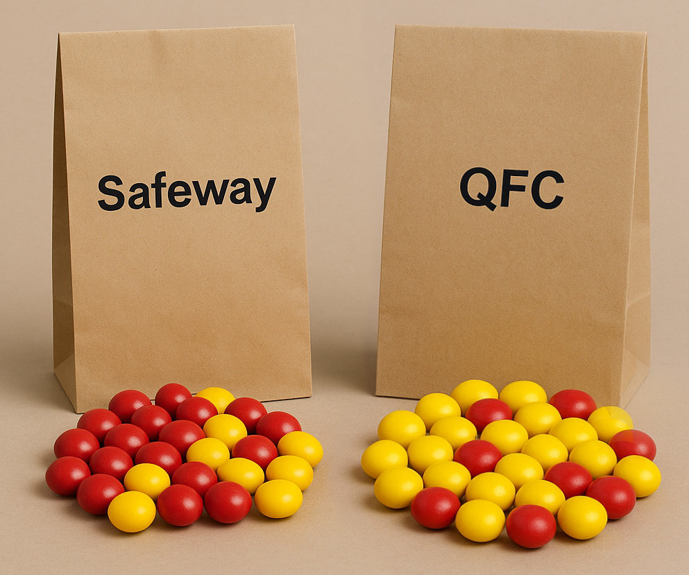
Which bag is from Safeway, which on from QFC?
Image by Zoe Huang, generated with ChatGPTObviously, you can pour the content out and immediately see if the candies are mostly red or mostly yellow. This is a fair way–it is comparable to asking every single voter whether they will vote for C or E. While you can do this with your M&M-s, this cannot be done with many many other interesting problems, and hence we do not talk more about such “brute force” approach.
Instead, imagine that you can only take a few candies out of the bag. The first candy you get happens to be red. Does it mean that the bag is bought from Safeway?
You are probably not that naive. Yes, Safeway bags contain more red candies, but there are also plenty of red ones in the QFC bags, and you can still, just by chance, get one from there.
Now you take out another candy, and this is red again.27 Can you now tell if this is from Safeway? Unfortunately still not. While everyone (including you) will probably agree that it seems to be the case, we cannot be certain. It is still possible that we get two red candies out of QFC bag, even if it is not that likely (the probability of Safeway is now 80% and of QFC 20%).
So how many red candies do we need to take out before we can be certain it is from Safeway? As it turns out, there is no such “many”. After three red candies, the odds are 8:1 (89% and 11%), after 4 red candies 16:1 (94% and 6%), after 10 red candies the odds that it is from Safeway are 1024:1 (99.9% and 0.1%) and so on. But there is never a point where you can be sure. True, if the bag is large enough, and if you by some inexplicable chance get 100 candies, all of which are red, the odds are \(2^{100}:1\), or about \(10^{30}:1\). The chance that it is bought from QFC is now approximately \(10^{-30}\), not zero, but the number is so small that it can be ignored for all normal decisions.28
This is the behavior of all statistical solutions. Statistics will never tell you that one answer is correct and another is wrong. It will tell you how likely each answer is. And you hope that one answer turns out to be “quite likely” while the others are “very unlikely”. In that case we can pick the likely one and hope for the best!
12.4.2 What are statistical hypothesis
Statistical hypothesis are in a sense extensions of the M&M example above. A hypothesis might be
A few comments about this hypothesis:H0: This bag is bought from QFC.
- Hypotheses are often denoted by “H”, followed by a number, often “H0”.
- The hypotheses are essentially “claims” about the world, and that sort of claims that can be analyzed with data.
- If is usually better to pick a claim that seems to contradict data. This is because when you find that the hypothesis is not compatible with data (you can “reject” it), then you have learned something. If it is compatible with data, you do not learn anything.
Let’s give now a more elaborate example using the same two bags of M&M-s.
Assume you got the bag from your friend, and without looking inside, you pull out 3 red candies from there. You’ll consider the hypothesis
H0: the bag is bought from QFC.
(QFC bags have 2/3 of yellow and only 1/3 of red beans.) The probability you get three red beans from the QFC bag29 is \(\left(\frac{1}{3}\right)^3 = \frac{1}{27}\) and the probability you get 3 red beans from a Safeway bag (where 2/3 are red) is \(\left(\frac{2}{3}\right)^3 = \frac{8}{27}\) (In most cases you’ll get some red and some yellow beans). Hence the odds of Safeway over QFC are \(r = \frac{8/27}{1/27} = 8\), or equivalently, the probability that the bag is from Safeway is \(\frac{8}{9} = 0.89\) and that it is from QFC is \(\frac{1}{9} = 0.11\). We can write these expressions using the common mathematical notation as \[\begin{align} \Pr(\mathit{Safeway}|R R R) &= \frac{8}{9} = 0.89 \\ \Pr(\mathit{QFC}|R R R) &= \frac{1}{9} = 0.11. \end{align}\] Where the first line reads “probability that the bag is from Safeway, given we sample three red beans” (that is what “RRR” stand for 😀). But what do the probabilities tell about the hypothesis and about the decision about which store the bag is from?
In statistics, we only consider a single decision: should we reject H0? We want to “reject” it if it is not compatible with data. And we make the decision based on its probability–if the probability is less than some kind of threshold, we will reject it, if it is over the threshold, we will not reject it.
Obviously, in order to reject, we need to decide the threshold. It is called significance level and often denoted by \(\alpha\). In social sciences, it is typically chosen \(\alpha = 0.05\), but sometimes also 0.1. In other sciences where datasets are much larger, one my chose much smaller \(\alpha\) in order to avoid type-1 errors (see Section 12.4.3). Importantly, significance level must be chosen based on the costs of different errors, not based on what you see in data.
Because guessing the store wrong will not bring large costs, we can pick a relatively large significance level \(\alpha = 0.1\). What will our decision be? Because \[\begin{equation*} \Pr(\mathit{QFC}|R R R) = 0.11 > \alpha \end{equation*}\] we cannot reject H0. This means we do not want to say that picking three red beans out of a QFC bag is incompatible with data. It is not very likely, but it is still compatible. Note that not rejecting H0 does not mean that H0 is correct! It just means that based on data, we cannot decide.
But now assume that you got four yellow beans from the bag, instead of three red ones. The odds now favor QFC as \[\begin{equation} \Pr(\mathit{QFC}|YYYY) = 0.941 \quad\text{and}\quad \Pr(\mathit{Safeway}|YYYY) = 0.059 \end{equation}\]
Exercise 12.1 Compute these probabilities!
How we may also want to test another hypothesis:
H1: this bag is bought from Safeway
Now the probability \[\begin{equation*} \Pr(\mathit{Safeway}|YYYY) = 0.59 < \alpha \end{equation*}\] and hence we can reject H1. But in a similar fashion as above, rejecting H1 does not mean it wrong. It just means that it is unlikely. Or more specifically–if H1 is correct, then it is unlikely to get four yellow beans from the bag, just by pure chance.
12.4.3 Type-1 and type-2 errors
As the decision to either reject or not reject a hypothesis can go wrong in both ways, we have two kind of errors.
First, we may by just be “bad luck” reject the hypothesis that is actually correct. In case of the four yellow beans from the bag we may reject H1: the bag is bought from Safeway, while it actually is brought from Safeway. We just be a rare chance get many yellow beans out of it.
This case is called Type-1 error or false positive. How often will you make type-1 errors in a large dataset? This is what the significance level \(\alpha\) is–if you are willing to reject the hypothesis if its probability is less than \(\alpha\), then there is still an \(\alpha\) chance that it is correct. This is the probability of type-1 errors.
Alternatively, we may fail to reject the hypothesis even if it is incorrect. This is called Type-2 error or false negative. It is more complicated to compute the corresponding probabilities because if the probabilities also depend on what is actually true, not just on our (incorrect) hypothesis.
Note that both types of errors are an inherent part of statistical decision-making. You do not make the errors not because you do it “wrong” or your calculations are “incorrect”. These errors are impossible to avoid because of the random noise in stochastic processes. So statistics can never give precise “yes” or “no” answers.
When making decisions to reject or not to reject the hypothesis, you should consider the costs of type-1 and type-2 errors. Sometimes one kind of error is much more costly than the other.
It may be confusing to remember what exactly is type-1 and what is type-2 error. Don’t worry. It does not matter much (unless you talk to a statistician). What matters is that you understand that the decisions can go wrong in two ways, and sometimes one way is much more costly than the other.
Exercise 12.2 You are working in a hospital with the task to analyze the patients’ blood samples to determine if they have cancer. Assume also that cancer is also a relatively rare condition among your patients.
- What might a suitable hypothesis \(H_0\) be?
- Given the hypothesis you picked above–what is a type-1 error and what is a type-2 error?
- Would you be more worried about type-1 errors or type-2 errors?
- Accordingly, what kind of significance level \(\alpha\), small (0.01) or large (0.1) will you choose?
12.5 Confidence intervals and statistical significance
One of the central concepts in statistical analysis are confidence intervals and statistical significance. In this section we’ll explain what do these two mean.
In the broad sense, confidence interval is the possible value range of the parameter that we have measured. You may have seen figures, presented using ±, for instance “the height of the tree is 72±1 m”. This is a way to display confidence interval–we know that the height of the tree can be anything between 71 and 73 m. But in statistics, the measure has a very specific meaning.
12.5.1 Confidence interval of values
Let’s start with looking not at a particular parameter but something else–the age distribution on Titanic (see also Section 10.2.1).
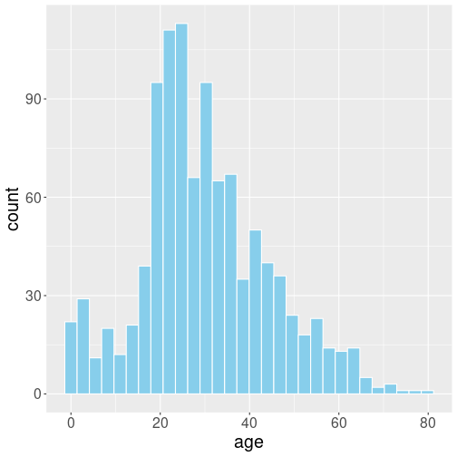
Titanic passengers’ age histogram.
The age histogram is presented at right. To make life easier, I removed the missing age values when loading data, so now we have 1046 passengers only but all of them have valid age.
titanic <- read_delim(
   "data/titanic.csv") %>%
   filter(!is.na(age))
titanic %>%
   ggplot(aes(age)) +
   geom_histogram(bins = 30,
                  fill = "skyblue",
                  col = "white")
Based on this figure, can you answer what is the “typical age range” of the passengers?
To begin with, the question is vague, so it cannot be answered precisely. But you’ll probably agree that “between 15 and 60” may be a suitable answer. But can we answer it in a more precise manner?
In order to provide a more precise answer, you need a more precise question. In statistics, it is common to ask
what is the age range that covers 95% of the passengers?
How can you answer this question? Well–you can order all passengers (1046) by age, remove the 2.5% (26) youngest ones and the 2.5% (26) oldest ones. In the sample that is left, the youngest and the oldest passenger represent such age range. This can be done using the tools we already know:
## Display the youngest 2.5% age:
titanic %>%
   arrange(age) %>%  # order by age in the growing pattern
   slice(1:27) %>%  # take off 2.5% plus one
   tail(1) %>%  # show the 'plus one'
   select(name, age)   # more clean printing
## # A tibble: 1 × 2
## name age
## <chr> <dbl>
## 1 Andersson, Miss. Ellis Anna Maria 2So the lower boundary of age is 2 years.
Exercise 12.3 Use the same method to find the upper boundary for the 95% age range.
However, in practice it is easier to use quantile functions. Quantile is a number that gives the boundary where 2.5% (or any other desired percentage) of values is smaller than the boundary and 95.5% are larger. This can be found as
titanic %>%
   pull(age) %>%   # extract 'age' as vector
   quantile(2.5/100)  # compute 0.025 quantile (2.5 percentile)
## 2.5%
## 2The lower 2.5th percentile is 2, exactly what we found above.
The quantile() function expects two arguments: first the data as
vector (see Section 3.6.3), here we use pipe to send
it. And second, the quantile. It wants the quantiles to be submitted
as percentages, so instead of percentile 2.5 we can use 2.5/100 to
get 0.025. quantile() also accepts a vector of quantile values,
so if you want to get both 2.5th and 97.5th percentile, you can call
##   2.5%  97.5%
##  2.000 61.875
So 95% of passengers were between 2 and 62 years old.
Exercise 12.4 Section 7.2.1.2 introduces median. What is median as a quantile?

We can mark these values on histogram as vertical lines:
titanic %>%
   ggplot(aes(age)) +
   geom_histogram(bins = 30,
                  fill = "skyblue",
                  col = "white") +
   geom_vline(xintercept = c(2, 62),
              col = "orangered")
It is hard to evaluate the exact percentages, but everyone probably agrees that most passengers fall between these two red lines.
This interval, 2 to 62 years, can be understood as the 95% confidence interval for the passengers’ age.30 It means that if you pick a random passenger from the boat, you can be 95% certain that their age falls into this interval. Or the way around–in only 5% of cases the age will be outside of this interval.
The way we built the 95% confidence interval (CI) above is not the only possible answer to “what is the age range of 95% of passengers”. Alternatively, you can take off the 5% of the oldest passengers, or maybe 5% of the youngest passengers instead. Those are called one-sided confidence intervals while above we constructed a two-sided confidence interval. Both have their uses, but the two sided CI tend to more common in applications. We do not discuss one-sided CI in this book.
Exercise 12.5 Construct the 90% confidence interval of the fare passengers paid. Display a similar histogram the includes the interval boundaries.
12.5.2 Confidence interval of sample average
Average age on Titanic
## # A tibble: 1 × 1
##   `mean(age)`
##         <dbl>
## 1        29.9
What is the range where 95% of mean age values fall?
What does this question even mean?
- Titanic had 1300 passengers and their average age was 29.9? No 95% here…
- If would like to let Titanic sail many times, each time it would have a different set of passengers with somewhat different average age. What is the 95% age interval?
- How can we calculate it?
Imagine a world of a very large number of “potential passengers”, where we have many who are in their twenties, and not that many who are below 15 or over 40. Each time Titanic sails, a random sample of them boards the boat.
Simulate this (bootstrap):
## [1] 29.9675## [1] 30.16149each time the results are slightly different.
## [1] 30.19925 29.96734 30.27040 29.77533 29.61393 29.80473 29.48279 28.67145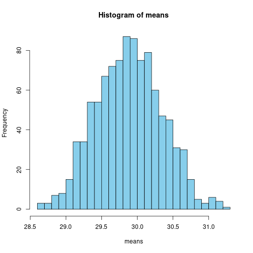 standard deviation:
## [1] 0.4595931This can be calculated mathematically using the Central Limit Theorem: \[\begin{equation} \frac{\text{std.dev}\; \text{age}}{\sqrt{N}} \end{equation}\] where \(N\) is the number of cases
## [1] 0.4456599Similar calculations can be done with most statistical values
HadCRUT temperature trend
hadcrut <- read_delim("data/hadcrut-annual.csv")
hadcrut %>%
   filter(Time > 1960) %>%
   lm(`Anomaly (deg C)` ~ Time, data = .) %>%
   summary()
##
## Call:
## lm(formula = `Anomaly (deg C)` ~ Time, data = .)
##
## Residuals:
## Min 1Q Median 3Q Max
## -0.22884 -0.09464 0.01395 0.07744 0.23983
##
## Coefficients:
## Estimate Std. Error t value Pr(>|t|)
## (Intercept) -3.593e+01 1.448e+00 -24.81 <2e-16 ***
## Time 1.819e-02 7.268e-04 25.02 <2e-16 ***
## ---
## Signif. codes: 0 '***' 0.001 '**' 0.01 '*' 0.05 '.' 0.1 ' ' 1
##
## Residual standard error: 0.1049 on 61 degrees of freedom
## Multiple R-squared: 0.9112, Adjusted R-squared: 0.9098
## F-statistic: 626.3 on 1 and 61 DF, p-value: < 2.2e-16hadcrut <- read_delim("data/hadcrut-annual.csv")
hadcrut %>%
filter(Time > 1960) %>%
lm(`Anomaly (deg C)` ~ Time, data = .) %>%
confint()## 2.5 % 97.5 %
## (Intercept) -38.82025626 -33.03025608
## Time 0.01673411 0.0196406295% confidence intervals: we are 95% certain that the true trend is between 0.0167 and 0.0196 deg C per year.
12.5.3 Linear regression and confidence intervals
When doing linear regression on real data, analysts are typically not just interested in the slope value, but also in the precision of the estimated value. This is done in various ways, often in several ways at the same time.
12.5.3.1 Regression table
Typically one prints out not just regression coefficients, but the
table of results. This can be achieved with the function summary().
Let’s compute here the temperature trend since 1961, replicating what
we did in Section 11.3.1. We use HadCRUT data
where Anomaly (deg C) represents the global temperature anomaly:
## # A tibble: 3 × 4
## Time `Anomaly (deg C)` `Lower confidence limit (2.5%)`
## <dbl> <dbl> <dbl>
## 1 1862 -0.536 -0.704
## 2 1861 -0.429 -0.597
## 3 1956 -0.263 -0.339
## `Upper confidence limit (97.5%)`
## <dbl>
## 1 -0.369
## 2 -0.261
## 3 -0.187And we compute the trend for post-1960 years. In Section 11.3.1 we did it as follows:
##
## Call:
## lm(formula = `Anomaly (deg C)` ~ Time, data = .)
##
## Coefficients:
## (Intercept) Time
## -35.92526 0.01819This tells that the global temperature is growing by 0.018 degrees each year.
In order to print the complete regression table, you just need to pipe
the result to summary() function:
##
## Call:
## lm(formula = `Anomaly (deg C)` ~ Time, data = .)
##
## Residuals:
##      Min       1Q   Median       3Q      Max
## -0.22884 -0.09464  0.01395  0.07744  0.23983
##
## Coefficients:
##               Estimate Std. Error t value Pr(>|t|)
## (Intercept) -3.593e+01  1.448e+00  -24.81   <2e-16 ***
## Time         1.819e-02  7.268e-04   25.02   <2e-16 ***
## ---
## Signif. codes:  0 '***' 0.001 '**' 0.01 '*' 0.05 '.' 0.1 ' ' 1
##
## Residual standard error: 0.1049 on 61 degrees of freedom
## Multiple R-squared:  0.9112, Adjusted R-squared:  0.9098
## F-statistic: 626.3 on 1 and 61 DF, p-value: < 2.2e-16- The regression coefficients -35.9 and 0.018 are in the column Estimate. The first one corresponds to the intercept (the row is labeled (Intercept), the second one corresponds to the slope Time. However, as their values are rather different, here they are printed in the exponential notation.
Pr(>|t|)denotes p-value, the probability that the null hypothesis is true (see below). As you can see, the probability is negligible for both intercept and slope.
Summary
sample: the information we collect about the process we want to analyze. Sample is often the same as “data”, this is what we know about the process.
sampling is the process that describes how certain cases end up in the sample. It is typically a stochastic process, where different cases may have similar or different probability to end up in the sample.
There are different ways of sampling:
- complete sample: include everything
- random sample: everyone has the same probability to be in the sample. This is the easiest sample to work with.
- stratified sample: “multi-level” sampling, for instance first you sample schools, and thereafter students withing the schools
- representative sample and biased sample: representative sample tend to give correct results; to get correct results with biased sample, you need to take into account the bias.
population: often it is only feasible to collect data (to measure) a small number of objects we are interested in. All the objects of interest together form the population. But there are processes where population is not about a large number, but about a certain properties insted.
12.6 Appendix: random numbers
R makes it easy to create a variety of random numbers and other random values. Here we discuss just a few: random integers, random values, and uniformly and normally distributed random numbers.
12.6.1 Random integers
Random integers can be created as sample(K, N, replace = TRUE).
This creates N
random integers between 1 and K. For instance, let’s create 10
integers between 1 and 3:
## [1] 2 3 2 3 3 2 1 2 2 2replace = TRUE means that all these numbers can occur more than
once. If you leave this out, then you’ll get an error in this case
because you cannot draw 10 different random numbers out of 1, 2, 3:
## Error in sample.int(x, size, replace, prob): cannot take a sample larger than the population when 'replace = FALSE'But another time you may need to ensure that every number is selected only once. For instance, if you want to allocate people to seats in a random fashion, then you only want to assign one person on each seat!
12.6.2 Other random values
sample() has a slightly different version where you can randomly
select any value, not just numbers \(1\dots K\). For instance
## [1] "B" "A" "A" "B" "B" "B" "B" "B" "B" "B"Will create a sequence of “A”-s and “B”-s, selected randomly.
Compared to how you can create random integers, this is mostly
similar. Just instead of the largest number \(K\), you need to supply a
vector of values, here c("A", "B"). The function c() creates
vectors, and "A" and "B" are the values you select from.
sample() has also other arguments, for instance you can select
different probabilities for different values.
12.6.3 Uniform random numbers
Uniform random numbers are fractions, uniformly distributed between 0
and 1. You can create \(N\) of those with runif(N). Here 5 uniform
random numbers:
## [1] 0.6589287 0.1262246 0.3052750 0.4971326 0.7210568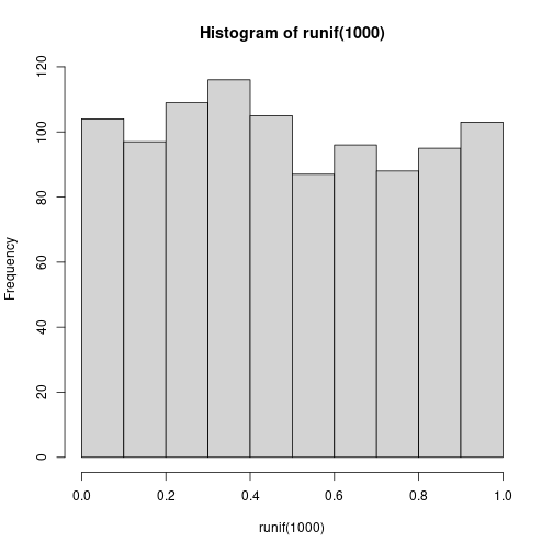
Histogram of 1000 random uniform numbers. They can have any value between 0 and 1.
If you make a histogram of these values, the result will look like a brick at right:
The histogram covers values from 0 to 1, and the bars that are about equal height show that different numbers in this range are equally likely.
See Section 10.2.1 for more about histograms.
12.6.4 Normal random numbers
Normally distributed random numbers are similar to the uniform ones in the sense that they can take any value. But unlike the uniform, they do not have a lower or upper limit. Instead, the values around zero are more common and the values further away increasingly less common.
You can create normal random numbers with rnorm(N), for instance,
here are five normal numbers:
## [1] 2.0429404 1.0126973 -0.7434544 -0.9344093 -0.4591088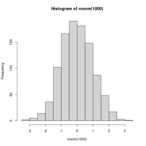
Histogram of 1000 random normal numbers. These can have any value, but values away from zero are increasingly less likely. This results in a well-known bell-shaped histogram.
The histogram of the normal numbers looks like the well-known bell curve:
In clearly reveals that most common values are near zero, but other values, both positive and negative, are also possible. On this figure, the smallest values are around -3.5 and the largest ones approximately +3.5.
12.6.5 Replicable random numbers
Random numbers are, well, random. If you want to generate these again, they end up being different. For instance, the first batch is
## [1] -0.9830526 -0.2760640 -0.8708510 0.7187106but the second batch is clearly different:
## [1] 0.11065288 -0.07846677 -0.42049046 -0.56212588This is sometimes exactly what you want–after all, there is little reason to make “random” numbers that are exactly the same. But other times this creates problems. For instance, if you want to discuss the smallest or the largest values, they tend to change each time you run your code, and hence you need to change the text accordingly each time.
As a solution, you can fix the random number seed. This is “initial
value” of the random numbers, and after fixing the seed, the numbers
come out exactly the same. Seed can be fixed with set.seed(S) where
S is a number–different S values correspond to different random
number sequences, but the same S value will always give you the same
numbers.
Here is an example where we generate two similar sequences of numbers. Pick seed 7:
## [1] 2.2872472 -1.1967717 -0.6942925 -0.4122930If you now just create a new sequence of numbers without re-setting the seed at seven, they end up different:
## [1] -0.9706733 -0.9472799 0.7481393 -0.1169552But if you want to replicate the first sequence, you can set the seed to seven again:
## [1] 2.2872472 -1.1967717 -0.6942925 -0.4122930Now the results are exactly the same as above.
TBD: create data frames
TBD: compute proportions
In statistics, one uses the concept of random variable to describe both populations, and such properties that can be computed from samples.↩︎
It would be better to call it uniform random sample, as “random” does not necessarily mean that everyone has the same probability.↩︎
We need to be a bit more specific here. As you already took out one red candy, there must now be fewer than 2/3 (Safeway) or 1/3 (QFC) of red candies. Hence the probabilities are now different. But let’s assume the bags contain a large number of candies (100 or more), in that case the difference is small and we can ignore it for now.↩︎
Just to give an idea how small is that number: the age of the universe, 13 billion years, is less than \(10^{19}\) seconds. You need to sample more than 100 billion bags per second through the whole lifetime of the universe, to have a realistic chance that you’ll hit one such bag from QFC.↩︎
The number of red and yellow beans you get (given the bags are large) follows binomial distribution.↩︎
However, one hardly uses the concept “confidence interval” to describe the distribution of observable data like age. This word is normally reserved for values you have to compute, like the average (see below), regression slope, or similar. But conceptually it is 95% confidence interval.↩︎