Chapter 5 More about data processing: dplyr pipelines

In these notes we are mainly using pipes for data processing. Pipes were introduced by magrittr package, and pipe-based workflows in dplyr package. Both of these are a part of tidyverse, so we do not have to do anything extra for loading these capabilities. Below we explain pipelines in depth using Titanic data so let’s load it right here:

library(tidyverse)
titanic <- read_delim("titanic.csv")

As a reminder, the dataset has

titanic %>%
   nrow()

## [1] 1309

rows and

titanic %>%
   ncol()

## [1] 14

columns, the first few lines of it look like

titanic %>%
   head(3)

## # A tibble: 3 × 14
##   pclass survived name                    sex      age sibsp
##    <dbl>    <dbl> <chr>                   <chr>  <dbl> <dbl>
## 1      1        1 Allen, Miss. Elisabeth… fema… 29         0
## 2      1        1 Allison, Master. Hudso… male   0.917     1
## 3      1        0 Allison, Miss. Helen L… fema…  2         1
##   parch ticket  fare cabin   embarked boat   body home.dest 
##   <dbl> <chr>  <dbl> <chr>   <chr>    <chr> <dbl> <chr>     
## 1     0 24160   211. B5      S        2        NA St Louis,…
## 2     2 113781  152. C22 C26 S        11       NA Montreal,…
## 3     2 113781  152. C22 C26 S        <NA>     NA Montreal,…

5.1 What are pipelines?

Pipes are a less-than-traditional way of feeding data to functions. Functions are the main workhorses of computing, they are the commands that can do all kinds of useful things, such as computing summary statistics and making plots. Functions are also widely used mathematical concept. Computer languages typically use syntax that is similar to mathematical functions. For instance, in math we write \[\begin{equation} \sqrt{2} \approx 1.414214 \end{equation}\] (square root of two–an irrational number–cannot be expressed exactly, hence written with \(\approx\) instead of \(=\)). But keyboards do not have square-root sign (and many other mathematical symbols), so on computers we traditionally write something like this:

sqrt(2)

## [1] 1.414214

This is similar to standard mathematical notation where functions are denoted like \(f(x)\) or \(g(z)\). We call \(2\), \(x\), and \(z\) function arguments and sqrt, \(f\) and \(g\) functions. So a function takes in arguments and does something with these, e.g. computes the square root, or maybe converts a text to upper case.

However, it turns out that for data processing, such an approach rapidly gets complicated to write, read, and think in. Instead, it is often (but not always!) useful to write arguments before the function. In R it looks like

2 %>%
   sqrt()

## [1] 1.414214

in mathematics, it would look something like \(x \rightarrow f\) and \(z \rightarrow g\) (but such notation is not common in math). In R, the second approach is exactly equivalent to the former, the traditional one.⁸ Why is the pipeline approach better? Well, it is not clear from this short example, but it is about reading and writing the code in the same way as you think about data processing. The logical order of operations in this example is this: 1) take number “2”; 2) compute square root of it. So the second approach is actually written in the order that we are doing things, sqrt(2) is not. But for this short example the difference may not be worth of the extra effort, sqrt(2) is clear and easy enough.

The special symbol %>% is called “pipe”.⁹ What pipe does it that it takes whatever was calculated at left of it, and feeds it into whatever is at right of it (or at the next line as we can break lines). So here the pipe means take “2” and feed it to the square-root function, so sqrt next to it will compute square root of “2”.

%>% is awkward to type. Use Ctrl-Shift-M in RStudio.

Why is this useful for data processing? Because we often need to do multiple steps with the same data, and we want to think, process, and read the code in a logical order. For instance, how do we compute average age of men who survived on Titanic? The recipe might look like this: 1) take Titanic data; 2) keep only males; 3) keep only survivors; 4) take their age; 5) compute the average. This is the logical order of doing things, some variations are possible, for instance, you can first keep survivors and then males instead the other way around. But you cannot first compute average age, and thereafter pick males. In this sense it is exactly like a cooking recipe. If you want to do pancakes, you have to start with eggs and sugar, and leave cooking for the last step. You can swap around the order of eggs and sugar, but you cannot do cooking before these two, and all other ingredients of the batter are in place.

The average age example can be written using dplyr pipelines as

titanic %>%  # take Titanic data
   filter(sex == "male") %>%  # keep only males
   filter(survived == 1) %>%  # keep only survivors
   pull(age) %>%  # take their age
   mean(na.rm=TRUE)  # compute the average

## [1] 26.97778

So we started by logical description of the data processing tasks, and translated it to code in a very similar fashion. This makes both reading and writing the code much easier. Another advantage of pipelines is that we can easily modify them. What if we are only interested in first class men? No problem, we just need to add something like 2.5) keep only first class passengers injected between the steps 2) and 3) above. In tidyverse parlance, we can write filter(pclass == 1) between lines 2 and 3.

Try to understand what is going on in these pipelines, and why they are so useful. At each step we take something we did earlier and modify it. For instance, filter(sex == "male") only keeps male passengers. We do this operation on Titanic data (the line above/before it) and pass the filtered data “down the pipe”. Downstream there is another filter: filter(survived == 1). This line only keeps the survivors of whatever comes into it. In the current case what comes in are the male passengers on Titanic, so the “flow” out of it contains just male survivors.

Below, we will discuss how to think, create and understand the pipelines, and what are the most important related functions. We also discuss how to debug pipelines, one of the major downsides of this approach.

5.2 Writing pipelines: split the tasks into small parts

Perhaps the most critical part of data processing (and many other tasks) is to be able to translate complex tasks into simple steps that can be implemented, either using pipelines or other tools. This may be a bit overwhelming for a beginner who does not know much about the available tools and their capabilities. Here we provide a few examples without any code. Afterward, in Section 5.3 we introducte the most important functions for such task.

Example 5.1 Let’s start with a simple question: How many second class passengers on Titanic did survived the shipwreck? Below is a potential tasklist:

1. take Titanic data
2. keep only 2nd class passengers
3. keep only survivors
4. how many do you have?

Obviously, there are other ways to approach it, for instance, you can swap around keeping the survivors and 2nd class only.

Exercise 5.1 Write a similar recipe for the question How many 3rd class women survived the Titanic disaster?

See the solution

Here is another example with Titanic data.

Example 5.2 Now we can ask the question Was the survival rate of men larger than that of women? This question is more complicated because we need to compute two survival rates, one for men and one for women. We can imagine something like that:

1. Take Titanic data
2. select only men
3. compute their survival rate
4. repeat the above for women
5. compare male and female survival rate.

This looks like a perfectly reasonable recipe, but now the knowledge of tools would help. First, how do we compute the survival rate? As the survived was coded as “1” for survival, “0” for death, we can just take the average of the survived variable. Second, here it is not really necessary to use computer to compare the values. Let the computer just print the two numbers, and humans can easily compare them. Finally, there are no good tools for “repeat the above for women”. Instead, there are good tools for “do the following for both men and women” (see Section 5.6). Knowing all these tricks, we want to write the recipe as

1. Take Titanic data
2. Do the following for men, women
3. keep only this sex
4. extract survived variable
5. compute its average

If done correctly, the computer will first keep only all women (because female is before male in alphabet) and compute their survival rate. Thereafter, it does the same for mean. We’ll get two numbers that we can easily compare.

Exercise 5.2 Make a recipe for this question: Which passenger class had the highest male survival rate?

Remember: there are three classes, 1st, 2nd and 3rd.

See the solution

Now let’s think about a different dataset. Now imagine that we have college data over a long time period, that contains students’ name, seniority (freshman/sophomore/…), id, and grades in info180, math126 and Korean103, year the grade was received, and the professor’s name.

Example 5.3 We may be interested if math grades have improved over time? Here we should perhaps compute math grade for each year, and then just compare the grades:

1. Take college data
2. Do the following for each year
3. pull out math126 grade
4. compute average

We’ll end up with a number of average grades, as many as how many years we have in a dataset. For a few years this is all well, but for, say, 35 years worth of data, we may want to add a final task, to make a nice plot of these averages (see Section 10).

As you can see, all other variables, such as professor’s name and grade in Korean are not relevant and we can just ignore those.

But sometimes the tasks are not that easy. We may need to define the concept much more precisely before we even can compute anything. Consider the following example:

Example 5.4 Which class–math or Korean–has seen more grade improvement over time? The problem here is that it is not immediately obvious what does “improvement” mean and how to measure it. There are a plethora of ways to do it, here let’s say that we simply compute the difference between the average grades for the last five and the first five years. We may consider something like this:

1. Take college data
2. keep only first 5 and last 5 years
3. Do the following separately for first 5 and for last 5 years:
4. Keep only these years
5. Compute average math grade
6. Compute average Korean grade
7. End of doing separately
8. Now compute difference between last math average and first math average
9. and between last Korean average and first Korean average

Note a few differences here: first, we still use the “do the following separately”, but now it is not for each year, but for certain groups of years. Second, we have stressed here that the last two lines–the differences over time–should not be done separately for the year groups. This is because we need both year groups to compute the difference, we cannot do it separately!

These were a number of examples about how to think in terms of splitting the task to small manageable parts. Next, we’ll look at the existing tools for doing this. We’ll start with basic dplyr functions.

5.3 The most important functions for pipelines

Dplyr pipelines are largely based around five functions: select, filter, mutate, arrange and summarize. Below we discuss each of these. But briefly:

• select: select desired columns (variables). Useful to avoid unnecessary clutter in your data, for instance when printing values on screen.
• filter: filter (keep) only desired rows (observations). Normally you provide it with various conditions, such as sex == "male", in this way we narrowed our example analysis down to just male survivors.
• arrange: order observations by descending/ascending order by some sort of value, e.g. by age.
• summarize: collapse data down to a small number of summary values, such as average age or smallest fare paid.
• mutate: compute new variables, or overwrite existing ones.

In the examples below we use the head function to show just a few first lines of the results. It is always advisable to frequently printing your results–in this way you understand better what you do and may spot problems early. But remember: head is not an organic part of most pipelines, it is a part of printing, the “situational awareness” of the process. You may want to remove it at the end.

5.3.1 Select variables with select

select allows one to select only certain variables. It is often desirable, in particular if you want to print some of your data. All too often there is too much irrelevant information that just clutters your document or computer window and obscures what is more important. So in most of the more complex tasks, one typically starts by narrowing down the variables.

In its simplest form, select just takes a list of desired variables:

titanic %>%
   select(survived, age, sex) %>%
   head(2)  # do not print too many lines

## # A tibble: 2 × 3
##   survived    age sex   
##      <dbl>  <dbl> <chr> 
## 1        1 29     female
## 2        1  0.917 male

Compare this with the printout of all variables–that would most likely not fit in your computer window, and obscure many values.

But there is a number of more advanced ways to use select. For instance, you can specify ranges using :, e.g. select(pclass:age) will select all variables from pclass to age (in the order they are in data, see introduction above):

titanic %>%
   select(pclass:age) %>%
   head(2)

## # A tibble: 2 × 5
##   pclass survived name                           sex   
##    <dbl>    <dbl> <chr>                          <chr> 
## 1      1        1 Allen, Miss. Elisabeth Walton  female
## 2      1        1 Allison, Master. Hudson Trevor male  
##      age
##    <dbl>
## 1 29    
## 2  0.917

Select also allows you to “unselect” variables using !. For instance, if we want to keep everything except name, we can do

titanic %>%
   select(!name) %>%
   head(2)

## # A tibble: 2 × 13
##   pclass survived sex       age sibsp parch ticket  fare
##    <dbl>    <dbl> <chr>   <dbl> <dbl> <dbl> <chr>  <dbl>
## 1      1        1 female 29         0     0 24160   211.
## 2      1        1 male    0.917     1     2 113781  152.
##   cabin   embarked boat   body home.dest                    
##   <chr>   <chr>    <chr> <dbl> <chr>                        
## 1 B5      S        2        NA St Louis, MO                 
## 2 C22 C26 S        11       NA Montreal, PQ / Chesterville,…

You can also rename variables when selecting as new = old:

titanic %>%
   select(name, class = pclass, survived) %>%
   head(2)

## # A tibble: 2 × 3
##   name                           class survived
##   <chr>                          <dbl>    <dbl>
## 1 Allen, Miss. Elisabeth Walton      1        1
## 2 Allison, Master. Hudson Trevor     1        1

Note that select selects the variables in this order. If you want to have the survival status before the passenger class in the final output, you may just swap the order of these variables in select, so you request select(name, survived, class = pclass).

Finally, a word about variable names. Normally you can write variable names in select in just the ordinary way, like select(name, age). But if variable names in data do not follow the R syntax rules (start with letter, and contain letter and numbers), then you may need to enclose the names in backtics `.¹⁰ For instance, if there is a variable called employment status (note the space in the name), then you have to write select(`employment status`).

There are many more options, see help for select, and R for Data Science.

Exercise 5.3 Print a sample of where you can see ticket price (fare) and passenger class (pclass). You can use sample_n() to get a sample.

What is the most expensive ticket you can see? In which class was that passenger traveling?

See the solution

Exercise 5.4

• Select only variables name, age, pclass and survived, in this order.
• Print a few lines of the result. You can use either head, tail or sample_n to print only a few lines.

See the solution

5.3.2 Filter observations with filter

5.3.2.1 Basics of filter

As select selects the variables (columns), so filter “filters” the rows. It requires you to specify one (or more) “filter conditions”, and only retains the rows where the condition holds (or all the conditions hold if more than one was specified). For instance, we can keep only passengers above age 60 by

titanic %>%
   filter(age > 60) %>%
   head(2)

## # A tibble: 2 × 14
##   pclass survived name                     sex     age sibsp
##    <dbl>    <dbl> <chr>                    <chr> <dbl> <dbl>
## 1      1        1 Andrews, Miss. Kornelia… fema…    63     1
## 2      1        0 Artagaveytia, Mr. Ramon  male     71     0
##   parch ticket    fare cabin embarked boat   body home.dest 
##   <dbl> <chr>    <dbl> <chr> <chr>    <chr> <dbl> <chr>     
## 1     0 13502     78.0 D7    S        10       NA Hudson, NY
## 2     0 PC 17609  49.5 <NA>  C        <NA>     22 Montevide…

If there are multiple conditions we are interested in, e.g. we only want to see survivors who were over age 60, then we can use two filter-s in a single pipeline:

titanic %>%
   filter(age > 60) %>%
   filter(survived == 1) %>%
   head(2)

## # A tibble: 2 × 14
##   pclass survived name                     sex     age sibsp
##    <dbl>    <dbl> <chr>                    <chr> <dbl> <dbl>
## 1      1        1 Andrews, Miss. Kornelia… fema…    63     1
## 2      1        1 Barkworth, Mr. Algernon… male     80     0
##   parch ticket  fare cabin embarked boat   body home.dest   
##   <dbl> <chr>  <dbl> <chr> <chr>    <chr> <dbl> <chr>       
## 1     0 13502   78.0 D7    S        10       NA Hudson, NY  
## 2     0 27042   30   A23   S        B        NA Hessle, Yor…

Alternatively, filter accepts multiple conditions, separated by comma:

titanic %>%
   filter(age > 60,
          survived == 1) %>%
   head(2)

## # A tibble: 2 × 14
##   pclass survived name                     sex     age sibsp
##    <dbl>    <dbl> <chr>                    <chr> <dbl> <dbl>
## 1      1        1 Andrews, Miss. Kornelia… fema…    63     1
## 2      1        1 Barkworth, Mr. Algernon… male     80     0
##   parch ticket  fare cabin embarked boat   body home.dest   
##   <dbl> <chr>  <dbl> <chr> <chr>    <chr> <dbl> <chr>       
## 1     0 13502   78.0 D7    S        10       NA Hudson, NY  
## 2     0 27042   30   A23   S        B        NA Hessle, Yor…

These two approaches are equivalent, so which one to use boils down to personal taste.

Note that testing for equality is done by double equal sign ==, not by a single sign! It is survived == 1, not survived = 1. It is a common mistake to use = instead of ==, in that case filter stops with a fairly useful error message:

titanic %>%
   filter(age > 60,
          survived = 1) %>%
   head(2)

## Error in `filter()`:
## ! We detected a named input.
## ℹ This usually means that you've used `=` instead of `==`.
## ℹ Did you mean `survived == 1`?

Another thing to know when specifying filters is that all literal text must be quoted. This includes all kinds of names and values that are not numbers. For instance, passenger names, the words such as “male” and “female”, and so on. For instance, selecting those who embarked in Southampton should be done with select(embarked == "S"), not with select(embarked == S). This is because the latter assume S is a variable name, and most likely complains that it cannot find such a variable:

titanic %>%
   filter(embarked == S)

## Error in `filter()`:
## ℹ In argument: `embarked == S`.
## Caused by error:
## ! object 'S' not found

Exercise 5.5 How many 3rd class male passengers were there?

Hint: use nrow to count the number.

See the solution

5.3.2.2 More about filter

Above we were just using the basic comparisons, == and >. But there are many more things we may want to do. Here is a list of more comparison operators you may find useful:

• ==: equality, as filter(survived == 1)
• >: greater than, as filter(age > 60)
• >=: greater than or equal, e.g. filter(age >= 60). This, unlike the previous example, will also include the 60-year olds.
• <: less than, as filter(age < 60)
• <=: less than or equal, e.g. filter(age <= 60). This, unlike the previous example, will also include the 60-year olds.
• !=: not equal. For instance, filter(embarked != "S") will keep everyone who did not embark in “S” (Southampton). So it only leaves passengers who embarked in “Q” (Queenstown) and “C” (Cherbourg).
• %in% c(...): only keep observations where the value is in a given list of values. For instance, if we want to keep everyone who embarked in Cherbourg (embarked = “C”) and in Queenstown (embarked = “Q”), then we can write filter(embarked %in% c("C", "Q")).

But all these comparisons may not be enough. Sometimes you also want to combine those, e.g. if a passenger was a male, and 20-30 years old, or alternatively, a female younger than 15. Such conditions can be combined using logical operators “AND”, “OR”, and “NOT”.

AND is the simplest operation to do with filter. For instance, the example above–a 20-30 year old man can be written as “passenger is a man and he is at least 20 years old and he is no more than 30 years old”. There are multiple ways how you can do this:

• You can combine three filter statements:

titanic %>%
   filter(sex == "male") %>%  
   filter(age >= 20) %>%   
   filter(age <= 30)

• Alternatively, you can use the AND operator &:

filter(sex == "male" & age >= 20 & age <= 30)

• In case of filter, you can just list multiple conditions, separated by comma. Filter treats multiple conditions as separate filter statements:

filter(sex == "male", age >= 20, age <= 30)

• There is also a helper function between, so you can write

filter(sex == "male", between(age, 20, 30))

All these options are equivalent, and it is about your taste and habit which one you want to use.

OR is another common operation. As separate filter conditions are treated as separate filters, one cannot do OR-operations by just separating arguments by commas. We need to use explicit OR operator | (the pipe).¹¹ For instance, to filter for “women, or anyone younger than 15”, we can do

filter(sex == "female" | age < 15)

Finally, NOT means to take everything, except the specified categories. The NOT-operator is !, normally you also want to put the condition in parenthesis. For instance, to select everyone who is not younger than 15, we can do

filter(!(age < 15))  # you may use 'age >= 15' instead  

The parenthesis are needed to speficy the exact order of operations. Here we want first to check if age is less than 15, and thereafter invert (NOT) the selection. If we leave out parenthesis, we first invert age, and thereafter compare the result with 15. This is normally not what you want.

In many situations, like in the example above, you do not need NOT. Instead, you can specify

filter(age >= 15)

These two approaches are equivalent. But in other contexts, NOT is a very handy tool.

5.3.3 Order results by arrange

arrange allows us to order data according to certain values. This is mostly used in case where we are interested in the largest or smallest values. For instance, who were the passengers who paid the smallest fare?

titanic %>%
   arrange(fare) %>%
   head(3)

## # A tibble: 3 × 14
##   pclass survived name                     sex     age sibsp
##    <dbl>    <dbl> <chr>                    <chr> <dbl> <dbl>
## 1      1        0 Andrews, Mr. Thomas Jr   male     39     0
## 2      1        0 Chisholm, Mr. Roderick … male     NA     0
## 3      1        0 Fry, Mr. Richard         male     NA     0
##   parch ticket  fare cabin embarked boat   body home.dest   
##   <dbl> <chr>  <dbl> <chr> <chr>    <chr> <dbl> <chr>       
## 1     0 112050     0 A36   S        <NA>     NA Belfast, NI 
## 2     0 112051     0 <NA>  S        <NA>     NA Liverpool, …
## 3     0 112058     0 B102  S        <NA>     NA <NA>

We can see that the cheapest fare is “0”.

But often we are interested in the highest fare instead. In that case we need to arrange data into descending order using a helper function desc as

titanic %>%
   arrange(desc(fare)) %>%
   head(3)

## # A tibble: 3 × 14
##   pclass survived name                     sex     age sibsp
##    <dbl>    <dbl> <chr>                    <chr> <dbl> <dbl>
## 1      1        1 Cardeza, Mr. Thomas Dra… male     36     0
## 2      1        1 Cardeza, Mrs. James War… fema…    58     0
## 3      1        1 Lesurer, Mr. Gustave J   male     35     0
##   parch ticket    fare cabin  embarked boat   body home.dest
##   <dbl> <chr>    <dbl> <chr>  <chr>    <chr> <dbl> <chr>    
## 1     1 PC 17755  512. B51 B… C        3        NA Austria-…
## 2     1 PC 17755  512. B51 B… C        3        NA Germanto…
## 3     0 PC 17755  512. B101   C        3        NA <NA>

The most expensive tickets were 512 pounds.

One can also order by multiple variables, in that case the ties in the first variable are broken using the second one:

titanic %>%
   arrange(desc(fare), sex) %>%
   head(3)

## # A tibble: 3 × 14
##   pclass survived name                     sex     age sibsp
##    <dbl>    <dbl> <chr>                    <chr> <dbl> <dbl>
## 1      1        1 Cardeza, Mrs. James War… fema…    58     0
## 2      1        1 Ward, Miss. Anna         fema…    35     0
## 3      1        1 Cardeza, Mr. Thomas Dra… male     36     0
##   parch ticket    fare cabin  embarked boat   body home.dest
##   <dbl> <chr>    <dbl> <chr>  <chr>    <chr> <dbl> <chr>    
## 1     1 PC 17755  512. B51 B… C        3        NA Germanto…
## 2     0 PC 17755  512. <NA>   C        3        NA <NA>     
## 3     1 PC 17755  512. B51 B… C        3        NA Austria-…

Now the passengers are first ordered by fare, but in case of equal fare, females are put before males (because “F” is before “M” in the alphabet).

5.3.4 Aggregate with summarize

summarize allows one to compute individual summary figures. These can be well-known summary statistics like mean or min, but they can also be other kind of things, e.g. count of words that begin with letter “A”. Just alone, summarize is not a very useful function (it is still useful though), but it becomes extremely handy when combined with grouped operations (see Section 5.6).

Summarize takes the form summarize(name = summary function). For instance, the mean age of all passengers is

titanic %>%
   summarize(mean(age, na.rm=TRUE))

## # A tibble: 1 × 1
##   `mean(age, na.rm = TRUE)`
##                       <dbl>
## 1                      29.9

summarize returns a data frame that contains a single row and one column for each summary statistic. As we asked only a single summary statistic–mean age–it only contains a single column. Also the variable name is perhaps somewhat inconvenient, it is literally the function we were using. We can rename it in a similar fashion as for select:

titanic %>%
   summarize(mean = mean(age, na.rm=TRUE))

## # A tibble: 1 × 1
##    mean
##   <dbl>
## 1  29.9

We can ask for more summary statistics by just adding the corresponding functions into the summarize:

titanic %>%
   summarize(min = min(age, na.rm=TRUE),
             mean = mean(age, na.rm=TRUE),
             max = max(age, na.rm=TRUE)
             )

## # A tibble: 1 × 3
##     min  mean   max
##   <dbl> <dbl> <dbl>
## 1 0.167  29.9    80

Now the resulting data frame still contains only a single line but three columns that are appropriately named as “min”, “mean”, and “max”.

5.3.5 Compute with mutate

mutate allows one to either create new variables, or overwrite the existing ones with new content. For instance, we can create a new variable child for everyone who is less than 14:

titanic %>%
   mutate(child = age < 14) %>%
   head(2)

## # A tibble: 2 × 15
##   pclass survived name              sex      age sibsp parch
##    <dbl>    <dbl> <chr>             <chr>  <dbl> <dbl> <dbl>
## 1      1        1 Allen, Miss. Eli… fema… 29         0     0
## 2      1        1 Allison, Master.… male   0.917     1     2
##   ticket  fare cabin   embarked boat   body home.dest  child
##   <chr>  <dbl> <chr>   <chr>    <chr> <dbl> <chr>      <lgl>
## 1 24160   211. B5      S        2        NA St Louis,… FALSE
## 2 113781  152. C22 C26 S        11       NA Montreal,… TRUE

Note the new variable child, the new variables are normally placed as the last ones in the data frame. There are many ways to do computations, and note that these do not have to be traditional mathematical operations. In the child example above, we were using a logical operation that results in either TRUE or FALSE, depending on if someone is younger or older than 14.

If you are not happy with TRUE-s and FALSE-s, one can also transform these into e.g. words “child” and “adult” using, for instance ifelse:

titanic %>%
   mutate(child = ifelse(age < 14, "child", "adult")) %>%
   head(2)

## # A tibble: 2 × 15
##   pclass survived name              sex      age sibsp parch
##    <dbl>    <dbl> <chr>             <chr>  <dbl> <dbl> <dbl>
## 1      1        1 Allen, Miss. Eli… fema… 29         0     0
## 2      1        1 Allison, Master.… male   0.917     1     2
##   ticket  fare cabin   embarked boat   body home.dest  child
##   <chr>  <dbl> <chr>   <chr>    <chr> <dbl> <chr>      <chr>
## 1 24160   211. B5      S        2        NA St Louis,… adult
## 2 113781  152. C22 C26 S        11       NA Montreal,… child

Now everyone who is younger than 14 is called “child”, and everyone 14 and above is “adult”. ifelse requires three arguments, a logical condition and two values–the first for TRUE and the second for FALSE cases.

5.4 Combining functions into pipelines

The power of these functions becomes apparent when we combine these into pipelines. For instance: what was the average fare paid by three oldest female survivors? Before we get to the code, we have to thing how to split this question into individual steps. These steps may look like:

1. take Titanic data
2. filter only survivors
3. filter only females
4. order by age in descending order
5. take top three rows of data (use head)
6. extract fare
7. compute mean

This can be implemented as

titanic %>%
   filter(survived == 1) %>%
   filter(sex == "female") %>%
   arrange(desc(age)) %>%
   head(3) %>%
   pull(fare) %>%
   mean()

## [1] 62.85277

So their average fare was 62 pounds.

Alternatively, we may ask what was their minimum and maximum fare paid. Now we want to learn two numbers, so we cannot use the exact same approach any more. We may want to return a data frame with these two numbers instead. Accordingly, the recipe would look slightly different:

1. take Titanic data
2. filter only survivors
3. filter only females
4. order by age in descending order
5. take top three rows of data (use head)
6. compute minimum and maximum fare (using summarize)

This can be implemented as

titanic %>%
   filter(survived == 1) %>%
   filter(sex == "female") %>%
   arrange(desc(age)) %>%
   head(3) %>%
   summarize(min = min(fare), max = max(fare))

## # A tibble: 1 × 2
##     min   max
##   <dbl> <dbl>
## 1  26.6  83.2

So the cheapest price they paid was 26 pounds, and the most expensive was 83 pounds.

Maybe we want to learn more about these passengers and just print their name, age, class and fare? No problem! We can just remove the summarize and add a select to avoid clutter and only display these variables: This can be implemented as

titanic %>%
   filter(survived == 1) %>%
   filter(sex == "female") %>%
   arrange(desc(age)) %>%
   head(3) %>%
   select(name, age, class=pclass, fare)

## # A tibble: 3 × 4
##   name                                                      
##   <chr>                                                     
## 1 Cavendish, Mrs. Tyrell William (Julia Florence Siegel)    
## 2 Compton, Mrs. Alexander Taylor (Mary Eliza Ingersoll)     
## 3 Crosby, Mrs. Edward Gifford (Catherine Elizabeth Halstead)
##     age class  fare
##   <dbl> <dbl> <dbl>
## 1    76     1  78.8
## 2    64     1  83.2
## 3    64     1  26.6

5.5 Other functions

5.5.1 Selecting rows

filter selects rows based on logical conditions, such as testing if age falls into a certain range. But sometimes we want to select rows based on position instead.

• head(n) selects the topmost n rows. This is useful if we have ordered data (using arrange) and now want to extract only rows with the largest or smallest values.
• tail(n) selects the last n rows.
• sample_n(n) selects a random sample of n rows. This is useful if we want to get a quick overview of everything, because the first and last rows in a dataset may not be quite similar to the rest of data.
• slice selects rows based on the row number. For instance, slice(1) takes the first row, the same as head(1). slice(1:5) takes the 5 first rows, like head(5). But slice(4:6) take rows 4, 5 and 6, something you cannot do by using just a single head.

For instance, we can answer the question how much did the 10th most expensive ticket cost? In order to answer this, we need

1. Order data by fare in descending order
2. extract the 10th row.
3. extract fare

We can do this by the following pipeline:

titanic %>%
   arrange(desc(fare)) %>%
   slice(10) %>%
   pull(fare)

## [1] 263

5.6 Grouped operations

A very powerful tool in the dplyr-framework is grouped operations. Essentially, grouping means splitting the dataset into groups according to a certain categorical variable (such as sex or pclass in case of Titanic), performing the desired operation separately for each group, and merging the groups afterward into a single dataset again.

5.6.1 Why grouping is useful

For instance, let’s compute the average ticket price (fare) for men and women. Without grouped operations, we can do it like this:

1. take Titanic data
2. filter males
3. compute average fare
4. take Titanic data
5. filter females
6. compute average fare

This approach is fairly easy, as we only have two values of sex. The tasks we do with each group, just compute the average fare, is simple too. For instance, for men we’ll find

titanic %>%
   filter(sex == "male") %>%
   summarize(fare = mean(fare, na.rm=TRUE))

## # A tibble: 1 × 1
##    fare
##   <dbl>
## 1  26.2

So men paid £26 for the ticket, in average.

But it is easy to imagine datasets where it is much-much harder to do such calculations. For instance, imagine you want to compute the yearly average temperature. The dataset you use, HadCRUT, contains just monthly temperatures. But unfortunately, it spans from 1850 till 2023. Good luck with repeating the above for 174 years! It is too tedious, and also rather error-prone. We should not copy the same code many times.

5.6.2 Single-column groups

This is where grouped operations come to play. Grouped operations is an additional tool–“do the following for all groups”. So we can write the pipeline above as

1. take Titanic data
2. do the following for all groups of sex:
   1. compute the average fare

This is it. We do not need to filter–“do this for all groups” will do the filtering for us, whatever the number of groups. It will also combine the results with the corresponding group identifiers. In computer code we can write the male/female average fare example as:

titanic %>%
   group_by(sex) %>%  # do the following for all groups of _sex_
   summarize(fare = mean(fare, na.rm=TRUE))

## # A tibble: 2 × 2
##   sex     fare
##   <chr>  <dbl>
## 1 female  46.2
## 2 male    26.2

We see that women paid more for the trip in average (approximately £46), than men (approximately £26).

The figure below gives explain how the grouped operations work.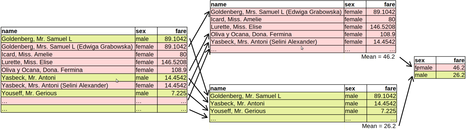

How grouped operations work: the dataset is split into groups (here female and male), the averages are computed separately for each group, and the results are combined again.

First, the Titanic data (left) is split into two groups based on the sex variable. Here the groups are female and male.¹² These two splits are now as good as two completely unrelated datasets. Next, the average fare is computed on both of these datasets. This results in two numbers, one for females, one for males. Finally, these two numbers are combined again, together with the corresponding group label. This is the final result of the commands above.

Exercise 5.6 Compute average fare by passenger class.

See the solution

Compute the survival rate by passenger class.

Hint: use mean(survived) for the survival rate.

5.6.3 Multi-column groups

So far we used just a single column to define the groups. But groups can be perfectly defined based on multiple criteria–for instance, based on sex and passenger class. This means that we will have all possible combinations of these two (or more) columns as the groups–we’d compute different values for 1st class females, 2nd class males, and so on. Technically, this can be achieved by just writing group_by(pclass, sex) for two-way grouping.

For instance, when you want to compute the survival rate by class and group, you can write

titanic %>%
   group_by(pclass, sex) %>%
   summarize(mean(survived))

## # A tibble: 6 × 3
## # Groups:   pclass [3]
##   pclass sex    `mean(survived)`
##    <dbl> <chr>             <dbl>
## 1      1 female            0.965
## 2      1 male              0.341
## 3      2 female            0.887
## 4      2 male              0.146
## 5      3 female            0.491
## 6      3 male              0.152

This reveals that 1st class women had very good chances to survive, while, unfortunately, for the 3rd class men the odds were almost 1 to 7.

Exercise 5.7 Above, in Section 5.6.2 we found that women paid more than men, in average. Why is it so? Is it because women were more likely to travel in upper classes? Find it out by computing male-female average price by passenger class.

The solution

5.7 Other pipeline tools

This section discusses selected other functions and tools that are useful when working with pipelines.

5.7.1 Renaming columns

In real-world datasets, you are frequently unhappy with certain column names. The actual names may be too long or too short, they may be not descriptive or they may be misleading, and they may contain characters that are hard to handle. Here are a few examples from real world data:

• time to denote year. I am again and again writing “year” instead of “time” and running into errors. Better rename it to year to begin with.
• 30. Thickness of ejecta in the distance of 10,000 m outside the rim [m]. Yes, this is a single column name (in a dataset about lunar craters)! It is way too long, and also contains too many special characters, including spaces, commas and brackets.
•   num_pages: it contains two space before text! It is hard to notice and hard to handle.
• اختصار جی پی اس: column names in languages that I do not speak using alphabet that I can neither read nor write.

Fortunately, columns can be renamed rather easily.

First, there is a dedicated function rename(). It should be used as a part of the pipeline in the form rename(new1 = old1, new2 = old2, ...) to rename a column called old1 to new1, old2 to new2 and so on. For instance, let’s rename the obscure sibsp column of titanic data into siblings:

titanic %>%
   select(name, sibsp) %>%
   rename(siblings = sibsp) %>%
   sample_n(3)

## # A tibble: 3 × 2
##   name                    siblings
##   <chr>                      <dbl>
## 1 Lahtinen, Rev. William         1
## 2 Assaf, Mr. Gerios              0
## 3 Wiklund, Mr. Karl Johan        1

Alternatively, you can rename columns using select(). The syntax is similar: select(new1 = col1, new2 = col2, ...). So we can achieve the same as above using

titanic %>%
   select(name, siblings = sibsp) %>%
   sample_n(3)

## # A tibble: 3 × 2
##   name                                               
##   <chr>                                              
## 1 Sjostedt, Mr. Ernst Adolf                          
## 2 Silvey, Mrs. William Baird (Alice Munger)          
## 3 Cumings, Mrs. John Bradley (Florence Briggs Thayer)
##   siblings
##      <dbl>
## 1        0
## 2        1
## 3        1

The difference between these approaches is that rename() preserves all columns, including those that you do not rename. select(), however, only keeps those columns that you explicitly select, using either the original or the new name.

5.7.2 Other

TBD: data=. in dplyr pipeline

5.8 Troubleshooting

Pipelines are easy and intuitive tools to think about data processing. But as with other tools, there are many things that can go wrong. Below is a brief list of problems that you may encounter, and some suggestions how to fix those.

5.8.1 Pipes at the end of pipelines

Pipes need something at both ends. At the left end of the pipeline you typically have a dataset, and at the right end you have some kind of summary or display function, such as summarize() or sample_n(). However, it often happens that you leave an “unattended pipe” at the end:

titanic %>% 
  filter(age < 14) %>%   # the pipe should not be here!

This code snippet first takes titanic data, thereafter filters all children, and then sends all the children to … nowhere.

Depending on how do you execute your script, it may either fail with Error: unexpected input, or not fail and just… nothing happens. But as in this example, actually something happens. Namely, RStudio expects that pipe leads to something–to another function, and is waiting for you to provide it. If this is the case, you see a + at the beginning of the last row. This is continuation prompt, marking that RStudio is expecting you to complete a previous command, and it is not ready for a new command. Among other things it means that RStudio will refuse to run your other commands while waiting.

If you indeed want to continue, then it is easy–just add whatever function you want to add there after the pipeline. If this was a mistake, just click on the console pane and press ESC to get rid of the continuation prompt. Thereafter you’ll see the normal prompt > again.

5.8.2 Pipe missing

You may have a spurious pipe at the end of the pipeline, but you may also forget to put pipe in the place where it is needed. For instance, suppose you want to filter all children on Titanic. But your command looks like

titanic  # a pipe missing!
  filter(age < 14)

This is essentially two separate commands. The first, titanic, will just print the titanic data. You will see a lot of output. The second one is filter(age < 15). What happens now will depend on how exactly does your environment look like. But quite likely you’ll see an error

Error: object 'age' not found

Technically, this means that the filter() command is going to look for a dataset or variable called “age” in your workspace (the “Environment” pane in RStudio, see Section 2.2). But quite likely you do not have such a variable, hence the error that ‘age’ not found.

More conceptually, this happens because you want to feed the dataset to the filter() command through the pipeline, but because you forgot to put pipe there, filter does not receive it and things that age < 14 is the data it has to work on.

5.8.3 Running only a part of pipeline

Cursor anywhere on the pipeline (here at the end) will run the whole pipeline. The results are visible on the console.

A common way to run just a section of the code is to highlight the desired section, and hit the Run-button (see Section 2.7) or Ctrl/⌘ - Enter (see Section C.1 for keyboard shortcuts). This is all well, except it may be hard to select the correct section of the commands–mouse is not made for such precision movement.

As a good alternative, you can hit the Run-button without any selection. If no code is selected, this command executes all code that is related to the current row. In case of pipelines, this means that RStudio will execute the whole pipeline because it understands that the multiple rows of code form a single command (the whole pipeline).

only a part executed

Alternatively, you can highlight the pipeline and hit the Run-button. If you highlighted the complete pipeline, it has the same effect as when selecting nothing. But if you miss a few lines or characters, it will result in an error.

5.8.4 Other problems

• tidyverse not loaded
• parenthesis must match
• comma before parenthesis
• missing pipes
• spurious pipes
• head at end of assignment

TBD: finish pipe troubleshooting.

TBD: explain the first argument, and how pipeline uses the first argument.

TBD: assignments

---

8. We can say that this is true in mathematics as well. Math is very much about definitions, and if we define that \(x \rightarrow f\) is equivalent to \(f(x)\), then, well, they are equivalent.↩︎

9. This is the most common magrittr pipe. There are more pipes.↩︎

10. On the U.S. keyboard, the backtick is normally located left of number “1”, together with tilde “~”.↩︎

11. On the U.S. keyboard, | is normally located at right, above “Enter” and right of “]”↩︎

12. Also, they are in this order: 1. female, 2. male. This is because by default, the groups are ordered alphabetically.↩︎