Chapter 10 Visualizing data
Data visualizations are a very powerful way to understand certain properties and relationships in data. They also may add a completely different feel to an otherwise dull report.
But visualizations are not all-powerful, and sometimes they can be even deceptive. Visualizations can usually represent only low-dimensional data (containing only 2-3 variables) well, the options to make a high-dimensional dataset visually understandable are very limited.
Different kinds of visualizations are useful for different type of data. Here is a list of some of the most important categories:
- Histogram: a single numerical variable. See Section 10.2.1.
- Scatterplot: two numerical variables. Scatterplot is the appropriate way to represent data points where there is no inherent connection between different points. See Section 10.2.2.
- Line plot: two numerical variables. Line plot is the appropriate way to represent data points where the data points are ordered, so there is a connection from the “previous” to the “next” point. See Section 10.2.3.
- Barplot: a categorical and a numeric variable, and you only want to show a single value for each category (e.g. mean income by occupation). See Section 10.2.4.
- Boxplot: a categorical and a numeric variable, but where you want to visualize the distribution of the numeric variable, depending on the category. See Section 10.2.4.
We discuss these visualizations in a more detail below.
R contains multiple ways to visualize data. This section relies ggplot framework. It is part of the tidyverse world, and hence does not require any additional setup.
10.1 ggplot visualization framework
ggplot is a framework designed for visualizing data. A ggplot plotting command consists of “layers”, separated by “+” sign. The most important layers are aesthetics, connecting data to the visual properties of the plot (e.g. instructing the computer to put variable “age” on the horizontal axis), and geoms, the layers that actually make a plot. Below, we provide a few basic examples, and discuss the plot types separately later.
We demonstrate the plots with Ice extent data and Titanic data. These can be loaded as:
Now we have loaded the datasets and stored it under names ice and
titanic in
the R workspace. The ice dataset looks like
## # A tibble: 3 × 7
##    year month `data-type` region extent  area  time
##   <dbl> <dbl> <chr>       <chr>   <dbl> <dbl> <dbl>
## 1  1978    11 Goddard     N        11.6  9.04 1979.
## 2  1978    11 Goddard     S        15.9 11.7  1979.
## 3  1978    12 Goddard     N        13.7 10.9  1979.
For now, the important variables are year, month, region, and area. Region means the hemisphere, “N” for north and “S” for south, area is the sea ice surface area (in millions of km²).
A simple scatterplot of ice area.
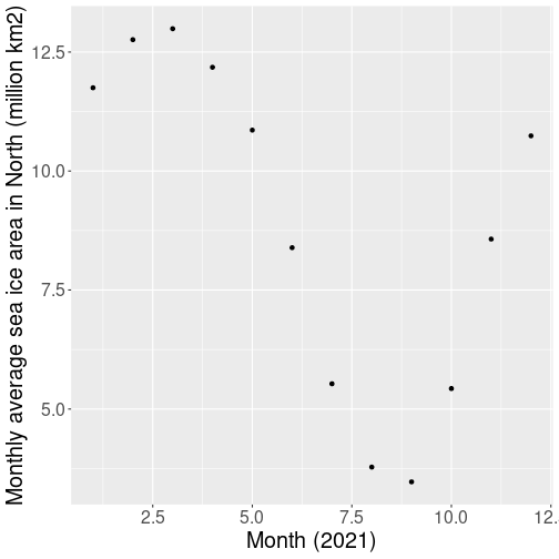
As an introductory example, let’s make a plot the sea ice area for each month for the northern hemisphere in 2021:
ice %>%
   filter(year == 2021,
          region == "N") %>%
               # only keep 2021 north
               # feed this to ggplot
   ggplot(aes(x=month, y=area)) +
   geom_point() +
   labs(x = "Month (2021)",
        y = "Sea ice area (M km2)")
The first three lines of the code just filter the 2021 northern
hemisphere data, and use the pipe %>% to feed this to ggplot().
Next, we get into the actual plotting:
ggplot()is the main plotting function. It can take many arguments, in this case the dataset (we feed data in through the pipe%>%) and the aestheticsaes().- Aesthetics,
aes(x=month, y=area))sets up aesthetics. This is the mapping between the visual layout of the plot, and variables in data. Here it tells that the variable “month” should be placed horizontally (as “x”) and “area” should be placed vertically (as “y”). But be aware that this line of code only sets everything up for plotting (such as axis, labels, and the gray background), but does not actually plot anything. - The third line,
geom_point()is the geom. Here we pick geom_point(), scatterplot, that actually makes the black dots that are visible on the image. - The final line,
labs(...)adjusts the axis labels. It is fairly self-explanatory. If you leave this out, the axis labels will be just the variable names, here “month” and “area”. - Note that the lines are combined with plus signs, not pipes. All the ggplot command is essentially a single command, you can think of the plus signs as the word “add”. The example above might then be read as
Take the ice data, filtered for year 2021 and northern hemisphere. Make a plot of it: put “month” on x-axis and “area” on y-axis. Add a scatterplot, add labels.
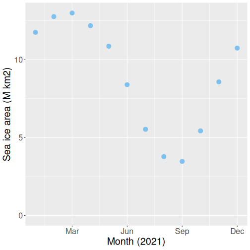
The same scatterplot as above, but now including more tuning.
ice %>%
   filter(year == 2021,
          region == "N") %>%
   ggplot(aes(x=month, y=area)) +
   geom_point(col = "skyblue2",
              size = 4) +
   labs(x = "Month (2021)",
        y = "Sea ice area (M km2)") +
   coord_cartesian(ylim = c(0, 13)) +
   scale_x_continuous(
      breaks = c("Mar" = 3, "Jun" = 6,
"Sep" = 9, "Dec" = 12))- Here we tell geom_point to make the points to be of color “skyblue2” (just search google for R color names, you can also use html hex values). We also request those to be larger (size 4).
coord_cartesian(ylim = c(0, 13))sets the vertical span of the plot to be from 0 to 13 (M km2). Here it is just to demonstrate the axis limits, but it also helps the reader to understand how far we are from zero–from no sea ice at all–condition.- Finally,
scale_x_continuous(breaks = c("Mar"=3, "Jun"=6, "Sep"=9, "Dec"=12))tells ggplot to only mark months 3, 6, 9 and 12, and label those not with the numbers, but with the month names.
Next, we’ll discuss the different plot types.
10.2 Basic plot types
10.2.1 Histogram
Histogram is a way to display distribution of a single variable. We encountered histograms in Section 7.2.3 above. It is essentially a frequency table of different values. For continuous variables, the values are binned, so we do not actually count the individual values, but instead, we count how many values fall into each bin. Histogram is a great way to display the distribution of the numeric variables.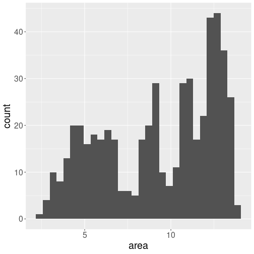
Distribution of ice area.
For instance, we can display the distribution of ice extent on northern hemisphere through all the years and months:
iceN <- ice %>%
   filter(region == "N") %>%
   filter(area > 0)
               # remove missings,
               # coded as negative values
ggplot(iceN, aes(x=area)) +
   geom_histogram()
The default values are not particularly beautiful–we have a number of dark gray bars on light gray background. But we can see that the values stretch from less than 3 to almost 15, with values around 12 and around 5 being the most common.
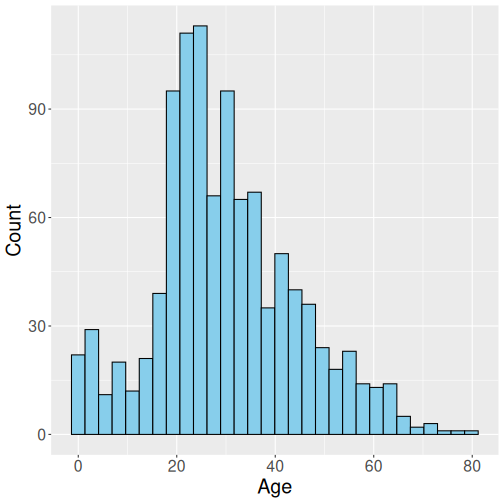
Titanic passengers’ age distribution
Let’s repeat it here again. First, load Titanic data:
titanic <- read_delim("data/titanic.csv")
ggplot(titanic,  # use 'titanic' data
       aes(x = age)) +
   geom_histogram(
      fill="skyblue",
      col="black",
      bins=30) +
   labs(x = "Age", y = "Count")
The code is largely similar to what we demonstrate above in Section 10.1. But a few differences are worth discussing:
- This time, we do not feed data to
ggplot()with pipe, but instead tell it what dataset to use (ggplot(titanic, ...)). - Histogram only needs a single aesthetic “x” (
aes(x = age)). This tells ggplot to make age histogram. - We ask to make the histogram bars with black borders (
col = "black") filled with skyblue color (fill = "skyblue"). Note that for histograms, barplots, and other plots that cover an area,fillmeans the fill color andcolmeans the border color. - We also ask for 30 bins.
- Finally, the better axis labels are added with
labs(), exactly as in Section 10.1.
Such a representation of passengers’ age is rather informative, for instance it tells that the bulk of passengers were between 20 and 40 years old, probably representing the prime age of settlers moving from the Old World to the New one. It also indicates another peak for toddlers, one may guess that this represents the children of the immigrants.
Why is histogram a good choice to visualize passengers’ age but not ice area? This is because passengers are independent entities, they do not transform to each other. This is not true for ice–for instance, March ice area will smoothly transition into April ice are, and then to May ice area. In such cases, histograms are much harder to interpret.
Exercise 10.1
- Imagine you have measured your height once every year. How would the corresponding height histogram look like?
- Repeat the exercise with your grandmother. How would the histograms differ?
- Can you learn anything interesting out of such height histograms?
10.2.2 Scatterplot
Scatterplot is a good way to relate two numeric variables. Above in Section 10.1 we used scatterplot (geom_point) to related time and ice area. Let’s do it here again, but now we will plot all months in data:
ice %>%
   filter(area > 0,  # exclude missings (marked as negative)
          region == "N") %>%  # only northern hemisphere
   ggplot(aes(time, area)) +
   geom_point(col="skyblue", size=0.5)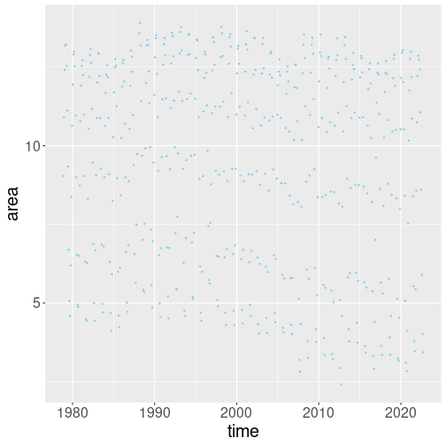
While this plot looks somewhat interesting, it is not very enlightening. The problem is that we are squeezing too much information–too many months with widely varying ice area–on the same plot. Let us just focus on a single month–September (month of the yearly northern ice minimum):
ice %>%
   filter(area > 0,
          region == "N",
          month == 9) %>%
   ggplot(aes(time, area)) +
   geom_point(col="skyblue3", size=3)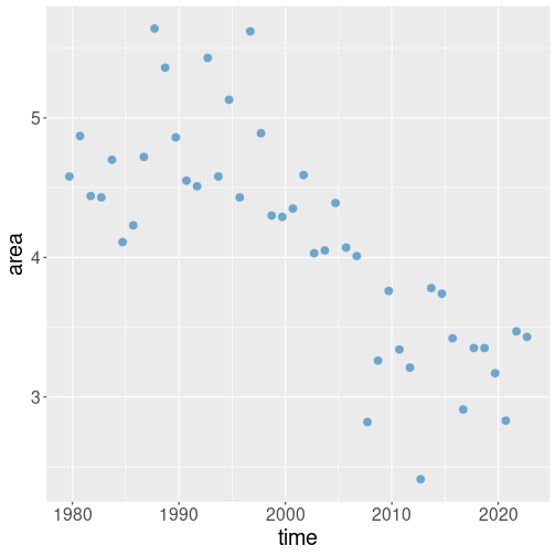
10.2.3 Line plot
Line plot is also a way to represent two numeric variables, in a sense it is very similar to scatterplot, but here the points (observations) must be somehow clearly linked, e.g. they may represent the same object measure at different point in time.
However, in case of ice extent over time, the points (years) are clearly ordered in time. Hence one may also consider connecting these with lines, transforming the plot essentially into a line plot:
ice %>%
   filter(area > 0,
          region == "N",
          month == 9) %>%
   ggplot(aes(time, area)) +
   geom_line(col="orangered") +
   geom_point(col="skyblue3", size=3)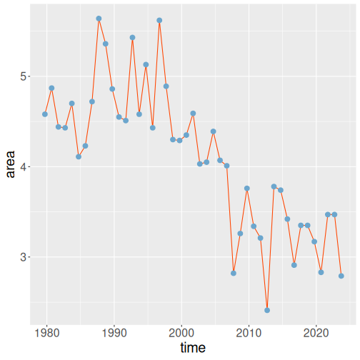
Here we use two geoms–geom_point to make the dots, and geom_line to connect them. Note that the geoms are drawn in the given order, here first the lines and thereafter the points. Here we are essentially using a combined plot, neither a pure line plot nor a pure scatterplot.
10.2.4 Barplot
Barplot is a way to display the relationship between a numeric and a categorical variable. Unlike in case of scatterplot and line plot, it is hard to display many different variables per category using barplot. For instance, we cannot really do a barplot of each fare paid by all the passengers depending on the class (but we can do such a scatterplot). Instead, we can make a barplot that shows the average fare paid on Titanic, by the passenger class. We start by computing the average by class:
## # A tibble: 3 × 2
## pclass fare
## <dbl> <dbl>
## 1 1 87.5
## 2 2 21.2
## 3 3 13.3(See Section 5.6 for more about grouped operations.)
This results in a data frame with two columns, pclass and fare. We can either store it as a variable, or feed directly to ggplot:
titanic %>%
   group_by(pclass) %>%
summarize(fare = mean(fare, na.rm=TRUE)) %>%
ggplot(aes(x=pclass, y=fare)) +
geom_col(fill="skyblue", col="white")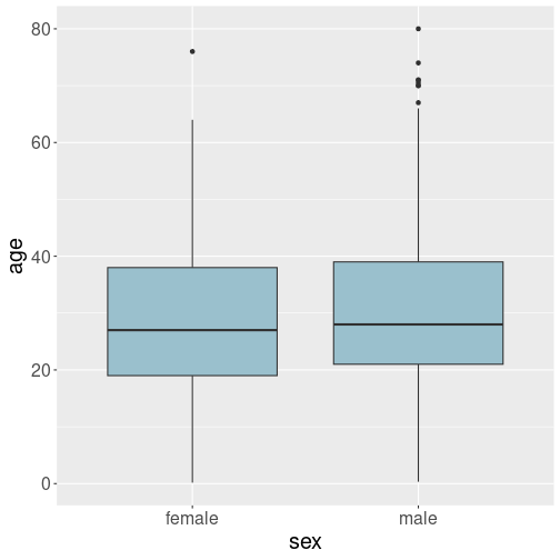
Why do we prefer a barplot here instead of scatterplot or line plot? Line plot would be quite misleading–the lines connecting the averages hint that there is some sort of continuous change from 87.5 (average for the 1st class) to 21.2 (average for the second class) and so on. But there is no continuous transition between classes.
Scatterplot is, strictly speaking, not wrong, but the small dots hint that these values are measured exactly at 1.0, 2.0, and 3.0 for the 1st, 2nd and 3rd class. It looks as if it is also possible to have 2.6th class and so on. Wide bars of the barplot stress that it is not possible.
10.2.5 Boxplot and violin plot
Boxplot is a way to compare distributions for different categorical variables. It is a little bit like several histograms, plotted next to each other, just the histograms are rather simplified. Boxplots are widely used in scientific literature, but not that much elsewhere.
Below, we compare the age distribution by sex. “Sex” (male and female) is a categorical variable, and “age” is a continuous numerical variable, distribution of which are we analyzing. One option for this is to do two separate histograms–one for men and one for women. This is, in essence, what boxplot does, just the histograms are very much simplified: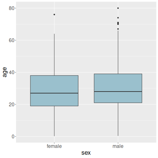
Boxplot to compare male and female age distributions.
Let us compare the age distribution of male and female passengers:
Typical boxplot shows multiple features of the distribution. The first, and the most prominent one, is the box. It displays where the most of data, from the first to the third quartile, is located. The thick black lines in the middle of boxes denote medians. We can see that the median age for both men and women is in the upper 20-s, slightly higher for men than for women. On top and bottom of the boxes are “whiskers”. These extend up and down by 1.5 times of the box height, but no further than the largest and smallest observation. Finally, data points that are further away than the end of whiskers are “outliers” and are marked as separate dots.
This plot shows that male and female age distributions are very similar. Men tend to be 1-2 years older than women, but no major difference is visible here.
Boxplot, as shown above, only works if the grouping variable is
categorical. Above, we use sex, that has two categories. However,
categories are often marked by numbers, and in that case R may just
not know that the variable is actually categorical. For instance, it
is common to denote sex by “1” and “2” instead of “male” and
“female”. In such cases we need to tell R that it is actually a
categorical variable by wrapping sex in the factor() function:
factor() changes the variable from numeric to categorical. Here it
is not necessary, because the existing categories are not numbers!
See more in Section 6.1.3.
Exercise 10.2 Make a box plot where you analyze the passengers’ age depending on their class. What can you conclude from this plot?
Hint: pclass is numeric, not categorical!
See the solution
Another plot type that can be used for the same tasks as boxplot is violin plot. They are called for violin plots because they typically look like some sort of elongated rounded symmetric objects, like violins.
Violin plots are almost like plotting multiple histograms, one for each group, vertically: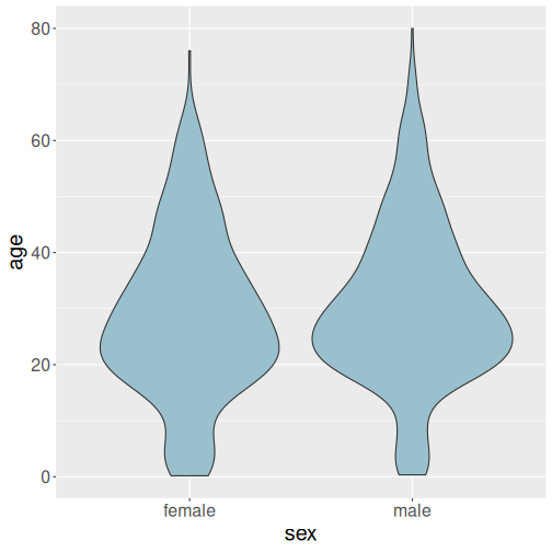
The same data as above, visualized as violin plot.
The violin plot gives us broadly similar information as boxplot. We can see that both men and women on the ship were dominatedly in their 20s and 30s, but there was also a number of children. We also see that men are somewhat older, but the difference is not large.
There are various options for violin plot, e.g. to display the sample quantiles.
Which one–boxplot or violin plot–should you choose? This depends on what exactly do you want to show. Do you want to show just a few sample quantiles? Then the boxplot is better, as it marks the quantiles and nothing else. But if you want to stress the shape of the distributions, then this is what violin plots are suited for.
Exercise 10.3 Create a violin plot that shows the ticket price (fare) as by passenger class.
See the solution
10.3 Grouping data on plots
A powerful feature of ggplot is to split the data into groups and denote the groups by different colors, line types or other markers.
10.3.1 Discrete grouping variables
Above, in Section 10.1, we made a plot of ice
area by month in northern hemisphere. We achieved this by first
filtering only northern values (filter(region == "N")), and second
by setting the month on the horizontal and ice area on the vertical
axis by aes(x = month, y = area). But what if we want to display
the amount on ice both in the southern and northern hemisphere?
region == "N" filtering
condition), and tell ggplot to use an additional aesthetic that will
now depend on the region. For instance, if we want to mark the
different hemispheres with different colors, we can add col = region
to the aes() function, so the function becomes
aes(x=month, y=area, col=region).
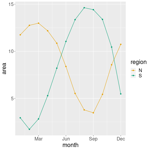
Here is the result:
ice %>%
   filter(area > 0,
          year == 2021) %>%
   ggplot(aes(x=month, y=area,
              col=region)) +
   geom_line() +
   geom_point() +
   scale_x_continuous(
      breaks = c("Mar"=3, "Jun"=6,
"Sep"=9, "Dec"=12))- month as horizontal position x
- area as vertical position y
- region as line color col.
The third aesthetic, col = region, is new. It functions in a very
similar way as x = month and y = area. The first part, col
tells to use an additional visual property color, and to connect it
to the data variable (column) region. So different regions should
be plotted with different color.
Note that col = region will automatically split the plot into two
separate lines, one orange (for north) and another green (for south). It
is not a single line with alternate red and blue segments! So
additional aesthetics not just make the points of different color,
they also separate the points into different groups. Even more, it
also adds the corresponding legend at the right hand side of the plot.
10.3.2 Continuous grouping variables
Now let’s do a different example. Let’s plot the northern monthly average ice area only.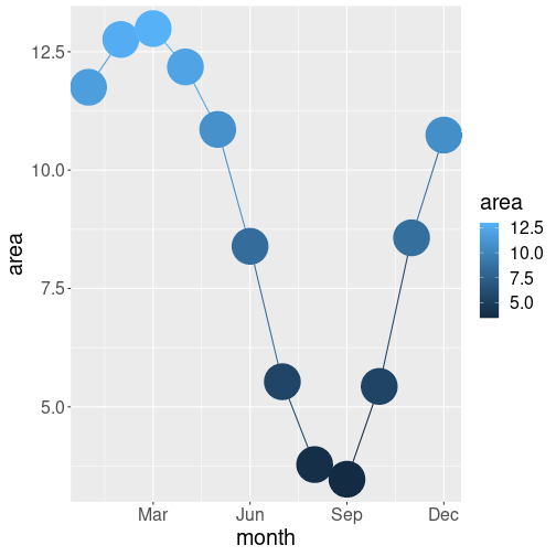
But this time, let’s color the points according to the area (also make them very large to be better visible):
ice %>%
   filter(area > 0,
          year == 2021,
          region == "N") %>%
   ggplot(aes(x=month, y=area,
              col=area)) +
   geom_line() +
   geom_point(size=15) +
   scale_x_continuous(
      breaks = c("Mar"=3, "Jun"=6,
"Sep"=9, "Dec"=12))- month as horizontal position x
- area as vertical position y
- area as the color for the points col.
So the only difference is that we colors the dots using area, not using region as above. But this results in quite a different plot.
First, we use the variable area for two different visual elements: vertical location and color. This is not a major difference, although it may look weird. It is perfectly fine, although somewhat redundant–we can guess what color is a point of based on its position, and we can guess its position based on its color. But this may be sometimes useful to stress a certain feature.
Second, and most importantly,
instead of making different lines for each area values,
we still have just a single line. Just the points are of different
color. Compare this with the previous example–when we requested col = region then we got two lines, now when we request col = area,
then we get a single line. Why is it like that? The reason is that
region is a categorical variable, but area is a numeric
(continuous) variable.
If you request the color (or other similar elements) to be dependent
on a categorical value, then the data points will be split into
different groups based on that value. If you request color to be
dependent on a simple numeric variable, then you get a single group,
but points are painted of different color. This is typically what one
wants, but sometimes this is not the case.

ice %>%
   filter(area > 0,
          month %in% c(3,6,9),
          region == "N") %>%
   ggplot(aes(x=year, y=area,
              col = month)) +
   geom_line() +
   geom_point()
The plot looks weird. Instead of three lines drawn in different colors, we see a single very jumpy line that contains dots of different shades of blue.
The problem is that our color variable, month, is not coded as categorical. If you look at a few lines of data,
## # A tibble: 1 × 7
##    year month `data-type` region extent  area  time
##   <dbl> <dbl> <chr>       <chr>   <dbl> <dbl> <dbl>
## 1  1978    11 Goddard     N        11.6  9.04 1979.
you can see that month is marked as <dbl>, i.e. a numeric
variable. Hence ggplot thinks it is a continuous number, similar to
area, that can take all sorts of values, including 1.5, 2.2, and
8.77432. And it prepares a set of blue colors to display all possible
values.
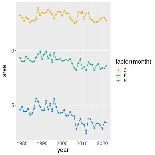
Fortunately, we can easily force a numeric variable into a categorical one using the function factor():
ice %>%
   filter(area > 0,
          month %in% c(3,6,9),
          region == "N") %>%
   ggplot(aes(x=year, y=area,
              col=factor(month))) +
   geom_line() +
geom_point()- year as horizontal position x
- area as vertical position y
- month as line color col. But because month is a numeric
variable, we convert it to a categorical one as
factor(month).
TBD: grouping data on plots exercises
10.4 Visualizing relationships
When visualizing data, we are very often interested in relationships.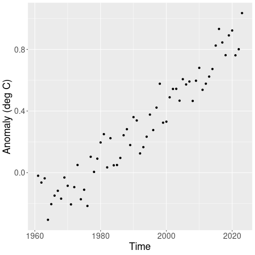
Relationship between time and global temperature.
Sometimes it is easy–for instance, the relationship between the global temperature and time using HadCRUT data (see Section B.2) is very easy to grasp even from a very simple plot:
hadcrut <- read_delim(
   "data/hadcrut-annual.csv")
hadcrut %>%
   filter(Time > 1960) %>%
   ggplot(
      aes(Time, `Anomaly (deg C)`)) +
          geom_point()
Everyone can immediately see a clear upward trend since 1960s.
TBD: smooth by averaging
But other time, the relationship is not so easy to visualize. Let’s take a more complex example–how does survival of Titanic passengers (see Section B.8) depend on age?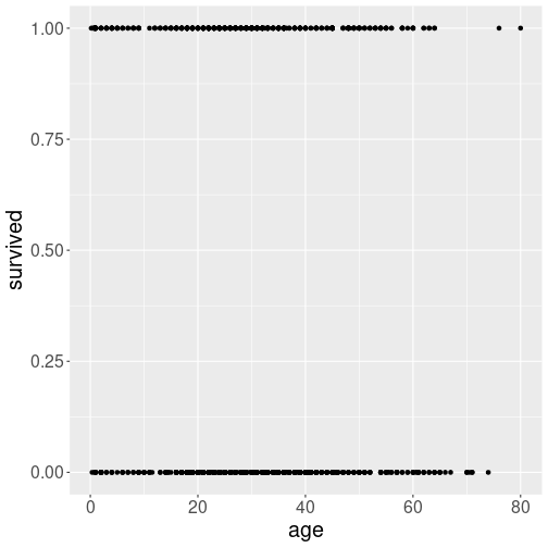
Passengers’ survival as a scatterplot
We may start with a similar approach as what we did above: just a simple scatterplot:
However, the result does not even resemble a plot. The main problem is that there are only two values for survival–either “0” (died) or “1” (survived). In an analogous fashion (but causing less issues), age is also in most cases coded as full years. Hence many points overlap and you cannot easily assess whether the trend is upward or downward.
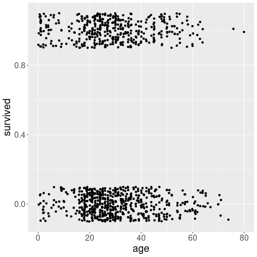
Survival as scatterplot, where the points are knocked off from their true location.
One potential solution to the overlaping points problem is to knock
the points off from their correct location in a random direction.
This can be achieved with geom_jitter() instead of geom_point().
We can also specify that we want the points to be moved up to 0.2
years left or right, and up to 0.1 up and down:
titanic %>%
   filter(!is.na(age)) %>%
   ggplot(aes(age, survived)) +
   geom_jitter(width = 0.2,
               height = 0.1)
The result is definitely better than above–at least we now have a good idea how many points there are–this information was impossible to read from the previous plot.
However, it is still hard to see how exactly the relationship depends on age.
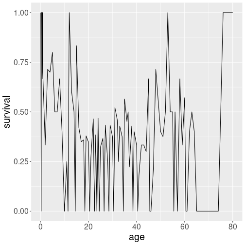
Average survival rate by ear of age.
In a naive fashion, one may want to compute the average survival rate by age:
titanic %>%
   filter(!is.na(age)) %>%
   group_by(age) %>%
   summarize(
      survival = mean(survived)) %>%
   ggplot(aes(age, survival)) +
   geom_line()
This works–sort of. But there are very few people of certain age, and hence the curve comes out too jumpy.
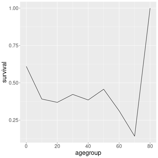
Average survival rate by 10-year age groups.
Let’s see how does it look when we make the plot by 10-year age groups:
titanic %>%
   filter(!is.na(age)) %>%
   mutate(agegroup = age - age %% 10) %>%
   group_by(agegroup) %>%
   summarize(survival = mean(survived)) %>%
   ggplot(aes(agegroup, survival)) +
   geom_line()
The plot finally looks quite clear!
There is another problem though: some of the age groups may have very few people only. In particular, there was just a single passenger who was 80. We may want to reflect the group size somehow on the plot. Even better, we may choose custom age groups instead of the 10-year interval applied uniformly to everyone.
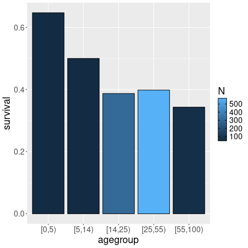
Survival rate by custom age groups, color denotes the group size.
This can be achieved using cut() function that cuts a continuous
variable (here “age”) into custom groups (see Section
6.1.6.2).
We pick age groups 0-5,
6-14, 15-25, 26-55, and 56-100. right = FALSE means that, for
instance, 5-year olds will belong to the left side group (0-5), not
the right side group (6-10). We can also use barplot where the color
denotes the group size.
titanic %>%
   filter(!is.na(age)) %>%
   mutate(
      agegroup = cut(
         age,
         breaks = c(0, 5, 14, 25, 55, 100),
         right = FALSE)) %>%
   group_by(agegroup) %>%
   summarize(survival = mean(survived),
             N = n()) %>%
   ggplot(aes(agegroup, survival,
              fill = N)) +
   geom_col(col = "black")
The result is pretty good. It indicates a downward trend–the two youngest age groups had higher survival chances than the other groups.
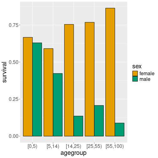
Male-female survival rate, displayed separately.
This can be achieved by specifying that the bars must be separated by, for instance, fill color:
titanic %>%
   filter(!is.na(age)) %>%
   mutate(
      agegroup = cut(
         age,
         breaks = c(0, 5, 14, 25, 55, 100),
         right = FALSE)) %>%
   group_by(agegroup, sex) %>%
   summarize(survival = mean(survived),
             N = n()) %>%
   ggplot(aes(agegroup, survival,
              fill = sex)) +
   geom_col(col = "black",
            position = "dodge")
This figure is very good in making it clear what happened to the boat–women and children were, indeed, much likely to survive.
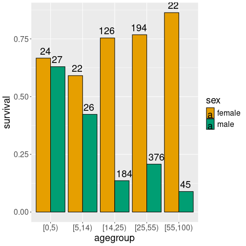
Male-female survival rate, and the corresponding group size.
This can be done with geom_text(), a similar plotting function like
geom_poin(), but instead of markers, it prints text, specified by
aes(label = N).
titanic %>%
   filter(!is.na(age)) %>%
   mutate(
      agegroup = cut(
         age,
         breaks = c(0, 5, 14, 25, 55, 100),
         right = FALSE)) %>%
   group_by(agegroup, sex) %>%
   summarize(survival = mean(survived),
             N = n()) %>%
   ggplot(aes(agegroup, survival,
              fill = sex)) +
   geom_col(col = "black",
            position = "dodge") +
   geom_text(aes(label = N),
             hjust = rep(c(1, -0.1), 5),
             vjust = -0.5)
Such plot involves some manual adjustment to get the labels at a suitable place. Here the main problem is that the female bars are plotted left, and the male bars right, so one has to adjust the female/male bars differently. By trial-and-error, I found that adjustment “1” is good for females and “-0.1” for males. As we have five bars, this pattern must be replicated for 5 times.
In terms of survival rate, the plot is the same as the previous one. However, it suggests that the two children groups and the elderly group were quite small, compared to the two group of adults.
These examples demonstrated a few ways to display the interesting relationships in data. Visualization is usually a good way to start your analysis, but not everything can be displayed with just scatterplots.