Chapter 4 Using R and RStudio for data analysis
In Section 2 we discussed how to install and run R, and how to load data. This section introduces a number of useful commands for basic data analysis.
4.1 Why R is useful?
Many beginners may find it hard to work with an environment that does not include menus and other “point-and-click” features. R is one such environment. Here we discuss briefly the advantages and disadvantages of such working environment.
Most work in R (and other similar environments) is done through
command (most of these are technically functions), such as
sqrt(2) or read_delim("file.csv"). In a way, this is not very
different from other environments, e.g. Excel or SPSS, except in those
program the functions can be accessed through the menus.
R does not offer such menus.6 There are several reasons for that.
- First, the sheer number of possible functions (depending on what exactly is installed, the number of functions may exceed 100,000). It will be too laborious to access the functionality through menus.
- Second, writing commands down (normally in the upper-left script window) is an excellent way to modify and repeat the operations. If you find that your first attempt to do the analysis was imperfect, then you can just modify the commands in the script window and re-run everything again. And when analyzing real data, we often need to do dozens or even hundreds of attempts before we are fully confident with our results. So being able to modify your commands is a critical tool that tremendously simplifies the analysis.
- Besides commands, one can also include comments in your scripts.
From the technical point of view, comments are just part of your
script that computer ignores (if R encounters
#on the line, it ignores the rest of it). So you can write anything you want there, even a poem if you wish. More likely, you want to explain what the script does, and why you have chosen to do it in a particular way. Such explanations are very handy both for you (as you will forget what did you do there) and also in case of your groupmates want to understand what did you do there. - Finally, commands written in the script window also form an excellent document of what was done. As these are the exact commands that were given to the computer, they also tell exactly what was done. Note that such document is hard to access in other environments, such as Excel, where the functions are not directly visible and previous commands can be overwritten by new results.
However, such a command-driven approach is not without its downsides. First, the commands are harder to discover (they are less “discoverable”). Good documentation, cheatsheets, and web search are needed much more often. And second–while the list of commands (code or “script”) tells exactly what to do, it also requires better understanding what happens when these commands are run. Spreadsheets, in contrast, show you immediately the effect of your commands and let you to analyze their results visually. While there are various techniques to improve the “situational awareness” when coding, it is not on par with the more visual tools.
4.2 How to think about data processing
A major part of any kind of data processing (and other analytic work) is to think and understand what you need to do. Data processing, in this sense, is like a cooking recipe. It is not enough to say “make a tasty curry”. You need to be able to translate the desired result (a tasty curry) into simple individual tasks. In case of curry, the translation might look like:
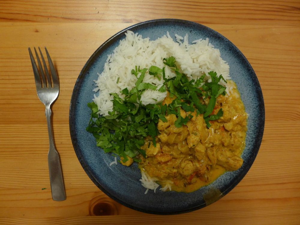
Data analysis is in some sense similar to cooking–you cannot just ask for a good dish. The road there goes through recipes, a precise list of steps you have to do in order to make the dish. For a successful data analysis, you need to come up with similar recipes.
- take two tablespoons of vegetable oil
- heat it in a deep pan
- add a cinnamon stick for 1 minute
- add 3 fresh bay leaves
- …
Being able to translate your desired result into such a recipe is one of the central skills for data processing (and for many other tasks). It does not matter much what kind of tools you are using–such a translation is needed in any case.
But how should the individual steps in the recipe look like? How simple or complex should they be? This depends on the tools you are using. Dedicated data processing environments typically have a plethora of powerful tools. Other times you have to get by with simpler ones. Again, it is similar to cooking–an experienced chef working in their own kitchen can easily figure out how what “cook meat until tender” means. But for a beginner, you may have to explain where to find the pan and what exactly is “tender”. So you have to know the tools you are using before you will be able to split your task into steps that are well suited for your tools.
4.3 The tidyverse world
As R is a very flexible language, it offers a wide variety of tools for the data analysis. In these notes we focus on the tidyverse approach. tidyverse is a set of packages (libraries), managed by Hadley Wickham, one of the main contributors of RStudio and an author of the excellent R for Data Science book.
This approach is focused on simplifying the traditional analysis through pipes and a limited set of functions. We touched this functionality briefly above in 3.7, now it is time to explain it in a bit more in depth.
4.3.1 Prepare for analysis
First, as tidyverse is not a part of the base R, we have to load it
explicitly to make it available for the current R session. (You need
to re-load it every time you close R.) This can be done using the
library function. But remember, before you can use library you
have to install the package, see Section
2.8. We load the library as
## ── Attaching core tidyverse packages ───────────────────────────── tidyverse 2.0.0 ──
## ✔ dplyr     1.1.4     ✔ readr     2.1.5
## ✔ forcats   1.0.0     ✔ stringr   1.5.1
## ✔ ggplot2   3.5.2     ✔ tibble    3.2.1
## ✔ lubridate 1.9.4     ✔ tidyr     1.3.1
## ✔ purrr     1.0.4
## ── Conflicts ─────────────────────────────────────────────── tidyverse_conflicts() ──
## ✖ dplyr::filter() masks stats::filter()
## ✖ dplyr::lag()    masks stats::lag()
## ℹ Use the conflicted package (<http://conflicted.r-lib.org/>) to force all conflicts to become errors
You can normally ignore the loading messages and the conflict warnings. Now everything is set up for the tidyverse functionality.
Finally, before we can get to examples, we also need to
load data. Below, we use read_delim() function,
but you can also use the data importer, see Section
3.7.
read_delim() is a
function that reads csv files, both comma- and tab-separated.
It can also figure out what is the correct separator. We
demonstrate the functionality using
Titanic
data
(See Section B.8).
as above:
Now we have loaded the dataset and stored it under name titanic in
the R workspace and we can take a look at it using commands.
4.3.2 Basic data description
In this section, the task is just introduce the approach used in tidyverse, see Section 5 for more in-depth explanation of the tidyverse functionality. Section 6 discusses the preliminary data analysis more in-depth with focus on the analysis, not on tools.
The way we work with data here can be thought as recipes in the form
- Take data
- Do something with these
- Do something more
- …
Here is an example: we want to know how many rows and columns is there in data. We can ask the rows as
## [1] 1309and columns as
## [1] 14Both of these can be understood as recipes, the first one to compute rows, and the second one to compute columns. We wanted two results, hence we need two recipes.
The %>% character is called pipe operator (see also Section
2.8). In takes what you did previously, and
feeds it into your next step. It is implicitly there in most cooking
recipes too–think about the recipe above: take two tablespoons of
vegetable oil %>% heat it in a deep pan %>% add a cinnamon stick for
1 minute…
Here we made
this explicitly with the pipe %>% between the stages, you can
read it along the lines “now take the result and next do
this:”.7
%>% is awkward to type. Use the keyboard shortcut Ctrl + Shift + M instead.
A few other tasks you may consider doing is to display a few lines of data. You can display a few first lines as
## # A tibble: 3 × 14
##   pclass survived name                           sex       age
##    <dbl>    <dbl> <chr>                          <chr>   <dbl>
## 1      1        1 Allen, Miss. Elisabeth Walton  female 29
## 2      1        1 Allison, Master. Hudson Trevor male    0.917
## 3      1        0 Allison, Miss. Helen Loraine   female  2
##   sibsp parch ticket  fare cabin   embarked boat   body
##   <dbl> <dbl> <chr>  <dbl> <chr>   <chr>    <chr> <dbl>
## 1     0     0 24160   211. B5      S        2        NA
## 2     1     2 113781  152. C22 C26 S        11       NA
## 3     1     2 113781  152. C22 C26 S        <NA>     NA
##   home.dest
##   <chr>
## 1 St Louis, MO
## 2 Montreal, PQ / Chesterville, ON
## 3 Montreal, PQ / Chesterville, ON
and a few last lines
## # A tibble: 2 × 14
##   pclass survived name                sex     age sibsp parch
##    <dbl>    <dbl> <chr>               <chr> <dbl> <dbl> <dbl>
## 1      3        0 Zakarian, Mr. Ortin male     27     0     0
## 2      3        0 Zimmerman, Mr. Leo  male     29     0     0
##   ticket  fare cabin embarked boat   body home.dest
##   <chr>  <dbl> <chr> <chr>    <chr> <dbl> <chr>
## 1 2670    7.22 <NA>  C        <NA>     NA <NA>
## 2 315082  7.88 <NA>  S        <NA>     NA <NA>
By default, only a few columns are displayed, no more than what fits to the screen. See Section 5.3.1 for how to display only variables-of-interest.
4.3.3 Working with individual variables
The above examples considered all the columns in the dataset. But sometimes we want to work with a single variable only. For instance, if you want to compute values, such as maximum fare, or create a frequency table of the passenger class, we need to extract individual variables. Here is an example of the latter:
## .
##   1   2   3
## 323 277 709
This example involves three lines. It can be read as “take Titanic
data; pull out the ‘pclass’ column; make frequency table of it”. Note
how the last line, table(), works not on the Titanic data (what we
have on the first line), but on the result of the second column
(separated pclass variable). We can make it explicit by removing
the last table() line (the output will be long though):
##   [1] 1 1 1 1 1 1 1 1 1 1 1 1 1 1 1 1 1 1 1 1 1 1 1 1 1 1 1 1 1 1
##  [31] 1 1 1 1 1 1 1 1 1 1 1 1 1 1 1 1 1 1 1 1 1 1 1 1 1 1 1 1 1 1
##  [61] 1 1 1 1 1 1 1 1 1 1 1 1 1 1 1 1 1 1 1 1 1 1 1 1 1 1 1 1 1 1
##  [91] 1 1 1 1 1 1 1 1 1 1 1 1 1 1 1 1 1 1 1 1 1 1 1 1 1 1 1 1 1 1
## [121] 1 1 1 1 1 1 1 1 1 1 1 1 1 1 1 1 1 1 1 1 1 1 1 1 1 1 1 1 1 1
## [151] 1 1 1 1 1 1 1 1 1 1 1 1 1 1 1 1 1 1 1 1 1 1 1 1 1 1 1 1 1 1
## [181] 1 1 1 1 1 1 1 1 1 1 1 1 1 1 1 1 1 1 1 1 1 1 1 1 1 1 1 1 1 1
## [211] 1 1 1 1 1 1 1 1 1 1 1 1 1 1 1 1 1 1 1 1 1 1 1 1 1 1 1 1 1 1
## [241] 1 1 1 1 1 1 1 1 1 1 1 1 1 1 1 1 1 1 1 1 1 1 1 1 1 1 1 1 1 1
## [271] 1 1 1 1 1 1 1 1 1 1 1 1 1 1 1 1 1 1 1 1 1 1 1 1 1 1 1 1 1 1
## [301] 1 1 1 1 1 1 1 1 1 1 1 1 1 1 1 1 1 1 1 1 1 1 1 2 2 2 2 2 2 2
## [331] 2 2 2 2 2 2 2 2 2 2 2 2 2 2 2 2 2 2 2 2 2 2 2 2 2 2 2 2 2 2
## [361] 2 2 2 2 2 2 2 2 2 2 2 2 2 2 2 2 2 2 2 2 2 2 2 2 2 2 2 2 2 2
## [391] 2 2 2 2 2 2 2 2 2 2 2 2 2 2 2 2 2 2 2 2 2 2 2 2 2 2 2 2 2 2
## [421] 2 2 2 2 2 2 2 2 2 2 2 2 2 2 2 2 2 2 2 2 2 2 2 2 2 2 2 2 2 2
## [451] 2 2 2 2 2 2 2 2 2 2 2 2 2 2 2 2 2 2 2 2 2 2 2 2 2 2 2 2 2 2
## [481] 2 2 2 2 2 2 2 2 2 2 2 2 2 2 2 2 2 2 2 2 2 2 2 2 2 2 2 2 2 2
## [511] 2 2 2 2 2 2 2 2 2 2 2 2 2 2 2 2 2 2 2 2 2 2 2 2 2 2 2 2 2 2
## [541] 2 2 2 2 2 2 2 2 2 2 2 2 2 2 2 2 2 2 2 2 2 2 2 2 2 2 2 2 2 2
## [571] 2 2 2 2 2 2 2 2 2 2 2 2 2 2 2 2 2 2 2 2 2 2 2 2 2 2 2 2 2 2
##  [ reached 'max' / getOption("max.print") -- omitted 709 entries ]
This is what the table() function works on afterward.
Otherwise, table() essentially just counts the “1”-s, “2”-s and
“3”-s. We can see that there was a comparable number of 1st and 2nd
class passengers, but the number of 3rd class passengers (709) exceeded the
combined number of the upper classes.
Exercise 4.1 What is minimum and maximum price paid by the passengers for the trip
(column fare)? Use a similar approach as above.
range(na.rm=TRUE) function will display both the minimum and maximum
price (na.rm ignores missing values, see Section
6.3 for more).
Comment what do you see.
See the solution
TBD: debugging
TBD: space inside of code
TBD: logical operations
TBD: strings in quotes
(Move to “pipelines”?)
RStudio includes menus, but those are limited to working with the script and the environment, very litte language functionality is accessible through RStudio menus.↩︎
Exactly as in recipes, not everything in data processing can be described as a single pipeline. For instance, in the curry you may actually need three pipelines: one for marinating the meat, the other for cooking it, and the third for cooking rice. In a similar fashion, you may need to use multiple pipelines in data processing.↩︎