Chapter 13 Logistic regression
In Section 11.3 we introduced linear regression, one of the most widely used tool to analyze relationships. Linear regression is an excellent choice for analyzing a large number of relationship–but not all of those. In particular, it requires that the outcome variable, \(y\), is continuous, or at least close to continuous. This was the case with both temperature, babies’ birth weight, and iris flower size. Note that the explanatory variable \(x\) does not need to be continuous, this was the case with the smoking example (Section 11.4.1).
However, for a large class of problems, the outcome is not continuous nor even a number. For instance, the question whether someone survived the shipwreck, whether a tweet will be retweeted, and whether an oil drill gets stuck in the drillhole cannot be described with continuous outcome. The passenger either survived or not, and a tweet was retweeted or not. Even if we describe these outcomes with numbers (e.g. survival as “1” and death as “0”), the result is not a continuous problem. We need different tools for this type of tasks. This is where logistic regression comes to play.
13.1 What is the problem with linear regression?
Consider policymakers during economically challenging times. Unemployment is large and work is nowhere to be found. Government is spending lot of money on benefits and the voices that are concerned about the effect on workers’ motivation and governments coffers are growing louder. But are the workers who are actually receiving the benefits? Does it actually affect their motivation?
Here we use benefits data. We focus on two variables: ui tells whether an unemployed person receives benefits (yes/no), and tenure is tenure at the job the worker lost, i.e. how many years did they work on that job. An example of the relevant data looks like
##    ui tenure
## 1 yes     21
## 2  no      2
## 3 yes     19
## 4 yes     17
This can be understood as the first worker applied for and received unemployment benefits, and they had been working for 21 years on the previous job. The second worker had been working on the previous job for 2 years, and did not apply for benefits.
But how is receiving benefits related to job tenure? One might guess that the longer time someone has been working at that position, the larger the potential benefits, and hence it is more worthwhile to apply. But is it actually the case? Let’s find it out!
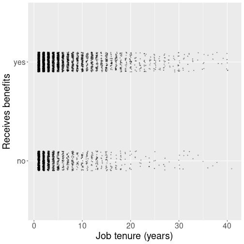
Receiving benefits as a function of job tenure.
A good place to start such an analysis is a plot. Put the receiving
benefits (“yes” or “no”) on the vertical axis and the
job tenure on the horizontal axis. We do the plot using
geom_jitter() to kick the points off a little from the only two
values (“yes” and “no”) in order to make them better visible
(see Section 11.4.2):
ggplot(Benefits,
       aes(tenure, ui)) +
   geom_jitter(height=0.1, width=0.2,
               size=0.5,
               alpha=0.3) +
   labs(y = "Receives benefits",
        x = "Job tenure (years)")
The figure reveals that at every year of tenure, it is common to see both those who receive and those who do not receive benefits. But it is hard to tell how these things are related–are benefits receivers more common among workers with less tenure, or among those with more tenure.
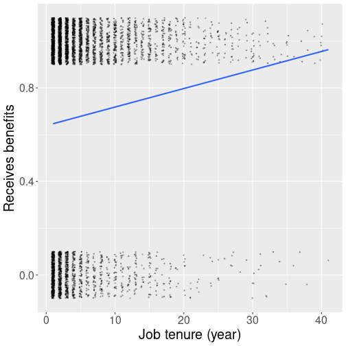
Receiving benefits as a function of tenure.
We can make the eventual trend visible
by adding a trend line.
For this to work, we need to convert the
variable on y-axis, ui, to a number (see
Section 11.4.1).
This can be done as
as.numeric(ui == "yes"):
Benefits %>%
   mutate(
      UI = as.numeric(ui == "yes")
   ) %>%
   ggplot(aes(tenure, UI)) +
   geom_jitter(height=0.1, width=0.2,
               size=0.5,
               alpha=0.3) +
   geom_smooth(method = "lm",
               se = FALSE) +
   labs(y = "Receives benefits",
        x = "Job tenure (year)")
The trend line is upward sloping. This means that those who have been working at the job for many years are more likely to claim benefits than those who have worked for a few years only.
But compare this plot with the on in Section 11.3.1 where we introduced linear regression. In that plot, the dots (global temperature anomaly) lined very well up with the trend line. Why is it not the case here? The culprit is the fact that the outcome is a binary variable. Benefit status can only be “yes” or “no” – “0” or “1” and nothing in between. Someone either receives benefits or does not receive benefits. But a line cannot touch just one or another of these values, a line also connects everything in between. So we necessarily see values like “0.1” and “0.5”, numbers that do not make any sense in terms of receiving benefits.
The way to overcome this problem is to interpret the outcome not as the outcome value–whether someone receives benefits–but the probability of the outcome, probability that someone receives benefits. So a value “0.5” would mean fifty-fifty probability that someone receives or does not receive benefits, while “0.99” means that the person almost certainly receives benefits. Taking this view, the trend line suggests that the probability for someone with 20 years of tenure to claim benefits is approximately 80%, but for a person with just one year of tenure, it is more like 55%.
In fact, this approach is widely used and a linear regression model that describes probability is called “linear probability model”. But linear probability models have another problem. You can see that the line exceeds unity around tenure 45. So how can we interpret the benefit probability of someone who has been working at the same job for all of their 50-year working life? It obviously cannot be more than 100%. In a similar fashion, the line will fall below zero somewhere (the tenure where this happens will be negative here, but in general, it is a similar problem). We can obviously hack the model in a way that we set probability to zero if the predicted probability is negative. But what should we now do with someone who has 48 years of tenure but does not claim benefits? If the participation probability at that tenure is 100%, then everyone should get benefits. Our model will be broken if it is not so. If you are still with me then you probably agree that making linear regression to work with probabilities needs a lot of hacks, and the model is not a nice and intuitive any more. So we need another to model the probability of benefits, not benefits; a way that ensures that the probability is always between 0 and 100%.
13.2 Logistic regression
There is a wide range of applications with binary outcomes where can such a model is handy. For instance, if someone attends college, gets a job, defaults a loan, that an email is spam, or that an image depicts a cat are all binary-outcome questions. And linear regression is not well suited to answer such questions.
Exercise 13.1
Would you use logistic or linear regression to analyze these questions:- How long will cancer patients survive after treatment?
- How good is students’ GPA?
- Who gets admitted to an elite school?
- Will the tweet be retweeted?
- How many people will read the tweet?
- Who survived a shipwreck?
13.2.1 Logistic function to model probability
Logistic regression (aka logit) is the most popular model designed for exactly this type of tasks, the tasks with binary outcome. “Binary outcome” means these questions only have two possible answers, either “0” or “1”, “true” or “false”, “cat” or “dog”, “raven” or a “non-raven”. This makes it distinct from linear regression that is designed to measure continuous outcomes, i.e. outcomes that can take all sorts of numeric values. Whether the outcome is coded as numbers or something else plays almost no role for logistic regression, we can always transform the two outcomes into “0” and “1”. This is what we did in the benefit example above where we converted “no” to “0” and “yes” to “1”.
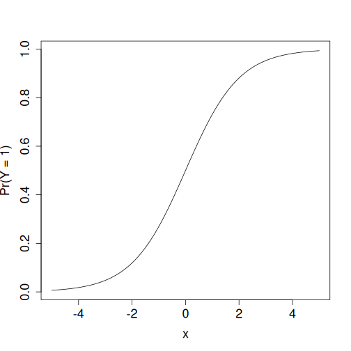
Logistic function: it transforms any number \(x\) into another number \(y\) between 0 and 1.
Mathematically, it can be done by using a function that transforms any number into and interval between 0 and 1. Logistic regression uses logistic function, \(\Lambda(x)\) (also called sigmoid function \(\sigma(x)\)): \[\begin{equation} \Lambda(x) = \frac{e^{x}}{e^{x} + 1} = \frac{1}{1 + e^{-x}}. \end{equation}\] The figure at right shows how any number \(x\) will be transformed into another number \(y\) that lies between 0 and 1–large negative numbers will be close to 0 and large positive ones close to 1. But they will never be below zero or above one. So logistic transformation produces results that can always be interpreted as probability.
Formally, one “embeds” the linear regression \[\begin{equation} y = b_0 + b_1 \cdot x p\end{equation}\] (see Section 11.3.4) inside the logistic transformation. So we compute the probability that the outcome occurs as \[\begin{equation} \Pr(Y = 1) = \frac{1}{1 + e^{-(b_0 + b_1 \cdot x)}}. \end{equation}\] So logistic regression is in many ways a similar model than linear regression–the model estimates two parameters \(b_0\) and \(b_1\), but instead of computing the outcome \(y\), it uses the parameters to compute the probability \(\Pr(Y = 1)\) for every data value \(x\).
This must be understood as the rule to compute the probability that the outcome \(Y=1\) if the value of the explanatory variable is \({x}\). Exactly as in case of linear regression, we have to find such parameters \(b_0\) and \(b_1\) so that the modeled probability will be the ``best’’ fit of data.
13.2.2 Logistic curve and probability in data

We can demonstrate this by choosing certain parameter values, and visually compare data with the predicted logistic curve. The purple curve at right uses values \(b_0 = 0\) and \(b_1 = 0.2\) and hence it computes \[\begin{equation} \Pr(Y = 1) = \frac{1}{1 + e^{-(0 + 0.2 \cdot x)}}. \end{equation}\] The visual inspection suggests that the curve is a bit too high, at least at the larger tenure values. True, there are more people with 30+ year of tenure who claim benefits, but while the curve claims the proportion is almost 100%, the visual inspection suggests it is much less. Hence the parameter values were not chosen well.
We can look at the case of people with 10-year of tenure. The probability, predicted by the logistic function is \[\begin{equation} \Pr(Y = 1) = \frac{1}{1 + e^{-(0 + 0.2 \cdot 10)}} = \frac{1}{1 + e^{-2}} = 0.88. \end{equation}\] We can compute the corresponding probability in data. Let’s take a slightly wider tenure range than exactly 10 years, for instance 8-12 years:
##          ui
## 1 0.7568966
So apparently the calculated probability is too large.
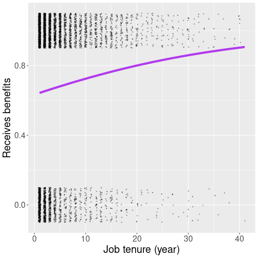
Here is another similar figure, but this time we have chosen \(b_0 = 0.547\) and \(b_1 = 0.042\) (these are actually the best logistic paramter values). Now the curve is much more flat, and it suggests that the probability of receiving benefits is nowhere as close to 1 as in the figure above.
And when you calculate the logistic probability, the result is much closer to that in data: \[\begin{equation} \Pr(Y = 1) = \frac{1}{1 + e^{-(0 + 0.042 \cdot 10)}} = \frac{1}{1 + e^{-2}} = 0.72. \end{equation}\]
13.2.3 What probability do you model?
But before we can even calculate anything, we have to specify which event are we modeling—are we modeling probability of benefits or non-benefits? In this case it seems more natural to model probability of benefits, i.e. to define \(Y = 1\) means receiving benefits and \(Y = 0\) means not receiving benefits. But it would be equally correct to specify it the other way around \(Y = 1\) means not receiving benefits. You have to choose.
In practice, it is often useful to specify that the “rare” event is \(Y = 1\), or that the probability of “intervention” is \(Y = 1\). Benefits does not check any of these boxes (in these data, 68% of people receive benefits), but it just feels more natural in this way. But whatever way you choose, be explain it clearly to your reader! It is unfortunately common to model the probability and not tell the readers what probability they talk about…
In practice, this decision is often let to the software, and the software often just orders the two categories alphabetically and picks the second one. So you your values are “0” and “1”, you’ll predict the probability of “1”, for “cat” and “dog” it will be “dog”, and for “male” and “female”, it will be “male”.
13.3 Logistic regression in R
R provides several ways to compute logistic regression. First I describe the dedicated info180 package, and thereafter the tools in base-R.
13.3.1 Logistic regression in info180 package
info180 is a dedicated package for this course. It is not available on CRAN (the R “app store”) and must be downloaded and installed separately. It is a compiled package, but its compilation does not require any special tools besides of R itself.
13.3.1.1 Installing info180
As it is not available on CRAN, you need first to download the package. Thereafter you can install it by issuing the command on the command prompt (see Section 2.2):
where"info180_0.0-4.tar.gz"is the name of the downloaded file (including the extensions), “0.0-4” was the most recent version during this writing. It should be in the same folder where your RStudio project (see Section 2.3). (you can also specify a correct path.)repos = NULLtells R not to go to internet to find a package with this name, but to look for such a package file locally.
After installation, you can use its functions in a similar fashion as we use tidyverse functions, by issuing
13.3.1.2 Performing logistic regression with logit()
Using info180, you can do logistic regression can be done in a fairly similar way as linear regression. The main function is
It will print the estimated parameters (\(b_0\) and \(b_1\)). Just be aware that you cannot interpret \(b_0\) and \(b_0\) just as intercept and slope in case of linear regression! (You need marginal effects, see Section 13.5).
Let’s use the logistic regression to model the benefits depending on job tenure. This can be done in the following fashion.
First, we focus on two columns in benefits data: ui (whether someone receives benefits or not), and tenure (job tenure in years). The former is coded as “yes” or “no”:
## .
##   no  yes
## 1542 3335
There are many more “yes”-s than “no”-s. If we rely on automatic ordering, logistic regression will model the probability of “yes”, as that follows “no” in alphabetic order. This is fine, as modeling the probability of benefits seems more natural here (at least to me).
We can run the logistic regression using
##
## Call:  glm(formula = formula, family = binomial(link = "logit"), data = data,
##     na.action = na.action)
##
## Coefficients:
## (Intercept)       tenure
##     0.54722      0.04205
##
## Degrees of Freedom: 4876 Total (i.e. Null);  4875 Residual
## Null Deviance:       6086
## Residual Deviance: 6025  AIC: 6029
This reports two coefficients: The intercept (0.547) and tenure (0.042). It is tempting to call the later “slope”, but it is not the slope of the logistic curve! So it cannot be interpreted in the similar fashion as how we interpreted the slope of linear regression (see Section 11.3.2).
13.4 Fix the draft text below
TBD: fix the messy logit text
pct30 <- treatment[age == 30, mean(treat)] @ For instance, let’s just guess that the values \(0\) and \(-0.1\) for \(\beta_{0}\) and \(\beta_{1}\) respectively, and compute the participation probability for a 30-year old person. We have \[\begin{equation} \label{eq:example-participation-probability-30-year-old} \Pr(T=1|\mathit{age}= 30) = \frac{1}{1 + \displaystyle\me^{-\beta_{0} - \beta_{1} \cdot \mathit{age}}} = \frac{1}{1 + \displaystyle\me^{-0 + 0.1 \cdot 30}} = \frac{1}{1 + \displaystyle\me^{3}} \approx 0.047. \end{equation}\] So our model, given the choice of parameters, predicts that rougly 5% of 30-year olds will participate. The actual number in data is . Figure~\(\ref{fig:logit-participation-age-trials}\) shows how the modeled participation probability depends on age for three different sets of parameters. The figure suggests that out of the three combinations displayed there, the one we calculated above \((0, -0.1)\) (blue curve) is close to actual data. The red curve \((0, 0.05)\) gets age dependency completely wrong, and the green curve \((0,-0.05)\) suggests participation probabilities that are too high. But it is hard to select good combination of parameters just by visual inspection even for this simple case with a single explanatory variable only. The best set of parameters for logistic regression is usually computed using Maximum Likelihood method (see~). The corresponding probability is shown by the dashed black curve.
When we compute the best possible coefficients (the dashed black line in Figure~\(\ref{fig:logit-participation-age-trials}\)), we get the following results: <<glm, results=“asis”>>= summary(m) %>% xtable() %>% print(booktabs=TRUE, include.rownames=TRUE, sanitize.rownames.function=latexNames) @ The results table, as provided by common software packages, looks rather similar to the linear regression table (see Table~\(\ref{tab:regression-table}\)). We see similar columns for estimates, standard error, \(z\)-value and \(p\)-value (obviously, different software packages provide somewhat different output). The meaning of the parameters is rather similar to that of linear regression with two main differences: first, the interpretation of logistic coefficients is quite different from that of the linear regression coefficients, so it is explained in the next section ().
Second, instead of \(t\)-values, logistic regression estimates are typically reported with \(z\)-values. From practical standpoint, these are fairly similar. Just instead of critical \(t\) value, we are concerned with critical \(z\)-values (for 5%-significance level it is 1.96, see Table~\(\ref{tab:t-values}\)). In a similar fashion, \(z\)-value measures distance between the estimated coefficient and \(H_{0}\) value, and in exactly the same way, the software normally assumes \(H_{0}: \beta = 0\). The difference between \(z\) and \(t\) values is primarily in the assumptions. In case of linear regression, for the \(t\) values to be correct, the error term \(\epsilon\) must be normally distributed. In logistic regression, for \(z\) values to be correct, the sample size must be large.
Logistic regression is in many ways similar to linear regression, including by being an interpretable model. Unfortunately, interpretation of logistic regression results is more complicated than in case of linear regression. There are two related reasons for that. First, logistic regression is a non-linear model, and hence the slope depends on the values of the explanatory variables (see Figure~\(\ref{fig:logistic-regression-interpretation}\)). And second, because the slope depends on the explanatory variables, we cannot just interpret the parameters \(\beta_{0}\) and \(\beta_{1}\) directly in terms of probability.
There are two popular ways to overcome these limitations: and .
13.5 Marginal effects
Marginal effect (ME) is slope of the logistic function on the figure where we have probability on the \(y\)-axis and the explanatory variable \(x\) (not the link function \(\eta\)) on the \(x\)-axis. Marginal effect answers the same question as slope \(\beta_{1}\) in case of linear regression: . In the example above, ME will answer the question . In case of multiple logistic regression we should also the add the phrase . So, in this sense marginal effects are very similar to linear regression coefficients. However, there are two major differences, both of these related to the fact that we now have a non-linear model:As marginal effect is just slope, we can compute it by taking the derivative of the logistic probability. For instance, in order to compute the marginal effect of age in the example above, we take derivative of the treatment probability~\(\eqref{eq:logit-treatment-age-link}\): \[\begin{equation} \label{eq:logit-age-marginal-effect} \pderiv{\mathit{age}} \frac{1}{1 + \displaystyle\me^{-\eta}} = -\frac{\me^{-\eta}}{ (1 + \displaystyle\me^{-\eta})^{2} } \beta_{1} \end{equation}\] where \(\eta = \beta_{0} + \beta_{1} \cdot \mathit{age}\). This is straightforward to compute, but normally we let statistical software do the work.
Figure~\(\ref{fig:logistic-regression-interpretation}\) demonstrates the meaning of marginal effects. The thick black curve is the logistic curve as a function of the link \(\eta\). Its slope differs at different points, here we have marked \(\eta_{1} = -2.5\) where the slope is \(0.069\), and \(\eta = 0.5\) where the slope is \(0.23\). These numbers—\(0.069\) and \(0.23\)—are the . But we are interested in instead–how much more likely it is to participate for those who are one year older. Now we have to take into account that \(\eta\) depends on \(x\) as \(\eta = \beta_{0} + \beta_{1} x\). Hence one unit larger \(x\) means \(\beta_{1}\) units larger \(\eta\) and hence the marginal effect of \(x\) is just the marginal effect of \(\eta\), multiplied by \(\beta_{1}\).
As marginal effects depend on \(\vec{x}\), we cannot just provide marginal effects that apply universally. Obviously, in case \(\eta\) is very small or very large, the effect will also be very small, while the \(\eta\) values near 0 are associated with larger effects. Typically, one of these three options is reported: Example of marginal effect output is in the table below:The basics of this table are quite similar to that of the logistic coefficients table above. is average marginal effect, software computes the marginal effects for every individual in these data and takes the average. stands for the standard error of , \(z\) and \(p\) are the corresponding \(z\) and \(p\) values, and the two last columns are CI for AME.
AME is directly interpretable in a similar fashion like the \(\beta\)-s in linear regression. The number \(\Sexpr{round(ame, 4)}\) means that: This can be phrased somewhat better using percentage points:And as explained above, if we are working with multiple logistic regression, we should add ``’’ to the sentence above.
13.5.1 Marginal effects with R
##    tenure
## 0.008986## lower upper
## tenure 0.006630047 0.01134163## factor AME SE z p lower upper
## tenure 0.0090 0.0012 7.4760 0.0000 0.0066 0.0113Another popular way to interpret logistic regression results is by using . Odds ratio is simply the ratio of the one group to the other, in the example above it will be the probability of participation over the probability of non-participation, \[\begin{equation} \label{eq:odds-ratio} r = \frac{\Pr(Y=1|\vec{x})}{\Pr(Y=0|\vec{x})} \end{equation}\] If we compute the probabilities using the sample averages, we get \[\begin{equation} \label{eq:odds-ratio-participation} r = \frac{N_{y=1}}{N_{y=0}} = \frac{ \Sexpr{sum(treatment$treat)} }{ \Sexpr{sum(!treatment$treat)} } = \Sexpr{ round(sum(treatment$treat)/sum(!treatment$treat), 3) }. \end{equation}\] Odds ratios are popular to describe the probabilities of certain kind of events, such winning chances in certain horse races. But unfortunately, these ratios are not used widely, and hence people tend not to understand the values well.
It turns out that logit coefficients are directly interpretable as effects on logarithms of odds ratios, . From~\(\eqref{eq:logistic-regression}\) we can express \(\me^{\vec{\beta}^{\transpose} \cdot \vec{x}_{i}}\) as \[\begin{equation} \label{eq:logit-odds} \me^{\vec{\beta}^{\transpose} \cdot \vec{x}_{i}} = \frac{\Pr(Y=1|\vec{x})}{1 - \Pr(Y=1|\vec{x})} = \frac{\Pr(Y=1|\vec{x})}{\Pr(Y=0|\vec{x})}. \end{equation}\] This is exactly odds ratio.
We can use this idea to find the effect on the odds ratio. Consider two vectors of explanatory variables, \(\vec{x}_{1}\) and \(\vec{x}_{2}\). The latter is otherwise equal to the former, except one of \(\vec{x}_{2}\) components, \(x_{2i}\), is larger by one unit compared to \(x_{1i}\). So while \(\vec{x}_{1} = (1, x_{11}, x_{12}, \dots, x_{1i}, \dots, x_{1K})\), the \(\vec{x}_{2} = (1, x_{11}, x_{12}, \dots, (x_{1i} + 1), \dots, x_{1K})\). Hence the odds ratio for case \(\vec{x}_{2}\) is \[\begin{multline} \label{eq:odds-ratio-effect} \frac{\Pr(Y=1|\vec{x}_{2})}{\Pr(Y=0|\vec{x}_{2})} = \me^{ \beta_{0} + \beta_{1}\,x_{11} + \beta_{2}\,x_{12} + \dots + \beta_{i}\,(x_{1i} + 1) + \dots + \beta_{K}\, x_{1K} } =\\= \me^{ \beta_{0} + \beta_{1}\,x_{11} + \beta_{2}\,x_{12} + \dots + \beta_{i}\,x_{1i} + \dots + \beta_{K}\, x_{1K} } \me^{\beta_{i}} = \frac{\Pr(Y=1|\vec{x}_{1})}{\Pr(Y=0|\vec{x}_{1})} \me^{\beta_{i}}. \end{multline}\] So \(\me^{\beta}\) describes the multiplicative effect on odds ratio: if \(x\) is larger by one unit, the odds ratio is larger by \(\me^{\beta}\) units. <<include=FALSE>>= ca <- coef(m)[“age”] eca <- exp(ca) ecaPct <- eca*100 ecaDiff <- 100 - ecaPct @ For instance, the age effect in the model~\(\eqref{eq:logit-treatment-age-link}\) above is . Hence the odds ratio effect is \[\begin{equation*} \me^{\Sexpr{round(ca, 3)}} = \Sexpr{round(eca, 3)}. \end{equation*}\] This means that odds of one year older individuals is times that of younger individuals. Or alternatively, one year older individuals have % lower odds to participate. Note that unlike in case of marginal effects, this number– %–is measured in percentages (of the baseline rate), not percentage points.
Odds ratios have two advantages over marginal effects: they are easier to compute (you only need to take exponent) and they are stable–odds ratios are constant and independent of personal characteristics. This contrasts to marginal effects that depend on the other parameters. But as odds ratios are harder to understand, and as nowadays the software to compute marginal effects is easily available, the odds ratios have become less popular.