Chapter 6 Preliminary data analysis
This section describes the first steps we usually take when starting working with a new dataset. The main message here is: understand your data.
6.1 Different variable types
We discussed the different kind of data in Section 3.2. That discussion was focused on data and how we understand it. Now we continue this discussion looking at computers and how computers represent it. Obviously, computer representation reflects of our understanding, but the details differ. For working with data on computers, it is important to understand the “computer’s mind”.
6.1.1 Numeric variables
One of the simplest data type is numeric.13 These are numbers of different kinds.
You can use the numbers as they are typically written to do common arithmetic operations:
## [1] 4.08## [1] 0.6666667## [1] 7## [1] 81By default, very large and very small numbers are printed in exponential form:
## [1] 2.409614e+13## [1] 4.154192e-11The first number must be understood as \(2.409614\times 10^{13}\) or \(24096140000000\), and the latter as \(4.154192\times 10^{-11}\) or \(0.00000000004154192\).
Exponential form can also be used to input large or small numbers:
## [1] 4400000## [1] 5.5e-09This is often easier to do
than to enter the numbers in the ordinary form as 4400000
and 0.0000000055.
If you load data in the tidyverse way, e.g. through read_delim()
(see Section 3.7),
the numeric columns will be marked as <dbl>. This means “double”,
standard double-precision numbers.
6.1.3 Categorical variables
Quite an important category are categorical variables, variables that represent values that are not numbers. In computer memory, these can be represented both as text, or as numbers.
If the numbers are represented as text, then all is well–R understands that text is not numbers, hence it is categorical. But when the categories are numbers, you may run into a trouble. The problem here is that R has no way of knowing if numbers are numbers (i.e. they can be added and averaged), or if they are categories (that cannot be added or averaged). For instance, in Titanic data (see Section B.8), the passenger class is coded as “1”, “2” or “3”. These are not numbers! These are categories. You cannot do mathematics like “first class + second class = third class”. This does not make any sense! However, they are stored in memory as numbers, and hence R, by default, treats these as any other numbers, and is happy to make all sorts of computations with these.
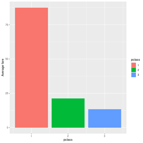
This causes problems when using certain functionality, e.g. plotting, where data handling depends on the data type. For instance, in case of categorical variables, we may want to color the different classes in clear distinct colors. The image here display the average fare on Titanic by passenger class. The classes are clearly distinct, depicted with very different colors.
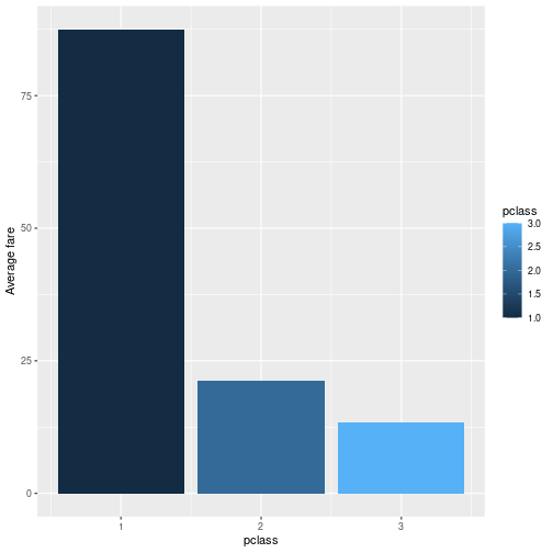
However, when R thinks that pclass is a number, it may display the colors on the same continuous scale instead. You can also see that the color key has middle values, such as 2.5 and 1.5. This is usually not what we want.
In such cases, one should convert the numbers to categoricals using
the factor() function. So instead of plotting average fare versus
pclass, you should plot average fare versus factor(pclass). See
more in Section 10.3.
6.1.5 Dates
A special data type is date. It is neither number nor character, it is, well, date. Dates are in many ways similar to ordered categoricals–we can tell if one date is “smaller” (i.e. earlier) than another, and we can find “minimum” and “maximum”, i.e. the earliest and the latest date. But unlike in the case of categoricals, the date differences can also be compared. For instance, we can say that the “difference” (time interval) between October 20th and October 30st is twice as long as between October 20th and October 25th.
6.1.5.1 Why dates are complicated
Although we may think that we understand dates well, the date as data type is actually surprisingly complicated. There are many reason for this.- To begin with, we need at least three different types of time measures–date, timestamp, and time interval. “Date” normally refers to a day, the whole day like “Sunday” or “my birthday”. “Timestamp” refers to precise time, including date and hours, minutes and seconds. And time interval is time difference, the duration, between two timestamps or between two dates.
- Second, there are no uniform way to represent dates. For instance, “Oct 19th, 2025” and “2025-10-19” are widely used and fairly unambiguous. But if you encounter date written like “5/1 2025” then you need to know if it is written according to the U.S. tradition (where it means May 1st), or the European tradition (where it means January 5th).
- Third, “date” normally refers to a day, a 24 hour interval. What do you think, does the Oct 19th (i.e. the 24 hours from Oct 19th 00:00:00 till 23:59:59) refer to the same time in Seattle and Shanghai? Are we talking about time-zone specific dates or dates in some kind of universal time? We need to decide.
- Fourth–casual computing with dates sometimes leads to weird result. What do you think–what should be the date one month ahead from January 30th? Should it be February 30th (which does not exist)? March 2nd (which sounds like two months ahead)? Or just we say it is NA–there is no such thing?
- Fifth: the only precise physical time unit is second. All others–minute, day, week, year can contain different number of seconds.
Unfortunately, there are many more problems, and hence working with dates is sometimes also complicated on computer.
Exercise 6.1
What data type: date, timestamp, or time interval would you use to describe- your friends’ birthdays (for instance, Jan 20, Mar 18, Oct 22)
- runners’ times (e.g. 1:20.3, 1:22.7, 1.25.1)
- time of sunrise and sunset (e.g. 7:02:13, 18:58:33)
TBD: finish the exercise
6.1.5.2 Loading dates
When you load a dataset that contains dates using read_delim() (see
Section 3.7), you may have the dates
automatically converted. But it depends on how exactly the dates are
coded. For instance, consider the following CSV file (see Section
3.6.2 for more about CSV files):14
## birthday     response     duration
## 6/12/2005    2025-10-19   22:27:25
## 1/2/2006     2021-11-01   14:33:14
## 7/3/2014     2020-08-02   9:12
This is a basic tab-separated CSV file with 3 rows and 3 columns: “birthday”, “response”, and “duration”. “birthday” is coded either as m/dd/yyyy or maybe d/m/yyyy; “response” is coded as yyyy-mm-dd (the standard ISO date format), and “duration” is coded as hh:mm(:ss). Out of these formats, only “date” is unambiguous. We cannot be certain if the first birthday refers to June 12th or 6th of December. The last duration may be either 9 hours 12 minutes, or maybe 9 minutes and 12 seconds.
We can load the dataset with read_delim():
## # A tibble: 3 × 3
##   birthday  response   duration
##   <chr>     <date>     <time>
## 1 6/12/2005 2025-10-19 22:27:25
## 2 1/2/2006  2021-11-01 14:33:14
## 3 7/3/2014  2020-08-02 09:12:00
The example shows that a) birthday is not converted in any way (it remains text “chr”; b) “response” in the ISO format is automatically converted to “date”; and c) “duration” is converted to time, assuming 9:12 means 9 hours and 12 minutes, the latter may or may not be correct.
Fortunately it is easy to convert birthday to “date” data type. Why do we want to do this? Because we may be interested in date arithmetic (see more in Section 6.1.5.3 below): to find the earliest/most recent date, to order data chronologically, or to compute time intervals between two dates.
We can
just use mutate() for computations
(see Section 5.3.5),
and then one of the special date functions, here
either mdy() for mm/dd/yyyy format or dmy() for dd/mm/yyyy
format. But before we do this, we need to know which format is the
birthday column using!
Assuming it is mm/dd/yyyy, we can write
## # A tibble: 3 × 3
##   birthday   response   duration
##   <date>     <date>     <time>
## 1 2005-06-12 2025-10-19 22:27:25
## 2 2006-01-02 2021-11-01 14:33:14
## 3 2014-07-03 2020-08-02 09:12:00
Now the birthday column is converted correctly. Note that “date”-type columns are always printed in yyyy-mm-dd ISO format.
Exercise 6.2 Convert birthday assuming it is coded as d/m/yyyy.
TBD: finish the date exercise
TBD: time interval data type
6.1.5.3 Arithmetic with dates
Date data type allows to perform simple but useful arithmetic. Most importantly, we can order time variables. The example date data can be ordered according to the response time as (see Section 5.3.3):
## # A tibble: 3 × 3
##   birthday   response   duration
##   <date>     <date>     <time>
## 1 2014-07-03 2020-08-02 09:12:00
## 2 2006-01-02 2021-11-01 14:33:14
## 3 2005-06-12 2025-10-19 22:27:25
or by by birthday, in decreasing order as
## # A tibble: 3 × 3
##   birthday   response   duration
##   <date>     <date>     <time>
## 1 2014-07-03 2020-08-02 09:12:00
## 2 2006-01-02 2021-11-01 14:33:14
## 3 2005-06-12 2025-10-19 22:27:25
Dates can also be used for simple filtering or otherwise comparison. For instance, you can list all records where birthday is after 2010:
## # A tibble: 1 × 3
##   birthday   response   duration
##   <date>     <date>     <time>
## 1 2014-07-03 2020-08-02 09:12
Note that here we wrote the date, Jan 1st 2010, as just a character
string. Those work perfectly, as long as it is in ISO format. If you
prefer something else, e.g. mm/dd/yyyy, you can use the same mdy()
function as in case of date conversion (see Section
6.1.5.2 above):
## # A tibble: 1 × 3
##   birthday   response   duration
##   <date>     <date>     <time>
## 1 2014-07-03 2020-08-02 09:12
6.1.6 Converting data from one type to another
TBD: need some kind of extra section for more computing details. TBD: move date conversion here?
It often happens that we are not happy with the original data type, so we need to know the ways how to convert one type to another.
6.1.6.2 Making categories out of numbers
One common problem with data is that they are numbers where we want or need categories. One such example occurs with plotting or certain other grouping, where we need to explain the computer that numbers “1”, “2” and “3” or not numbers in the mathematical sense that cannot be added or multiplied. Section 6.1.3 discusses one such case where these numbers are passenger classes where 1st class plus 2nd class does not equal 3rd class.
In such cases, one can easily explain R that the corresponding classes
are categories by using the factor() function: this just makes
categories out of numbers (or texts). For instance, in the original
data
## # A tibble: 3 × 2
##   name                           pclass
##   <chr>                           <dbl>
## 1 Allen, Miss. Elisabeth Walton       1
## 2 Allison, Master. Hudson Trevor      1
## 3 Allison, Miss. Helen Loraine        1
you can see that pclass is a number “<dbl>”. The converted pclass, however, is factor “<fct>”:
## # A tibble: 3 × 2
##   name                           pclass
##   <chr>                          <fct>
## 1 Allen, Miss. Elisabeth Walton  1
## 2 Allison, Master. Hudson Trevor 1
## 3 Allison, Miss. Helen Loraine   1
(See Section 5.3.5 for more about
mutate().)
Another, a very different reason is that often we do not want as detailed information as the numeric variables provide. We want a few categories instead. For instance, instead of a variable age that spans from 0 to 100, you may want to analyze a few groups only: “children”, “adults” and “elderly”. Or instead of education spanning from 0 to 20 years, you may want to have a few categories, such as “high school”, “college”, “graduate degree”. Here we explain one way how to achieve this, and example usage for data visualization is shown in Section 10.4.
Let’s convert the Titanic passengers’ age into three group: “children”
(0-13 years old), “adults” (14-50 year olds) and “elderly” (51 and
above). This can be achieved by the function cut(). It takes in a
column (a data vector, see Section 3.6.3) and the
conversion boundary specification (another vector),
and creates the corresponding
categories. We can specify the boundaries, for instance, as c(0, 13, 50, 1000):
## # A tibble: 4 × 3
##   name                        age agegroup
##   <chr>                     <dbl> <fct>
## 1 Lahtinen, Rev. William       30 (13,50]
## 2 Assaf, Mr. Gerios            21 (13,50]
## 3 Wiklund, Mr. Karl Johan      21 (13,50]
## 4 Sjostedt, Mr. Ernst Adolf    59 (50,200]
The boundary specification creates three groups (note that you need four boundaries for three groups). The first group will be from 0 to 13, and is denoted as “(0, 13]”, the second group “(13, 50]” is from 13 to 50, and the last, “(50, 200]” is from 50 till 200. As the latter is beyond anything like a realistic age, it is effectively equivalent to “above 50” (you can also start the first group not from 0, but from -1, to denote any age below 13.).
However–such conversion has an issue. If you specify that the first
boundary should be at 13, then what should we do with 13-year olds?
Will they be “children” or “adults”? By default, they are considered
to belong to the higher group (i.e. the right-hand boundary of the
interval is included in the interval). This is denoted by the
standard group labels, “(” in “(13, 50]”
means that the number “13” is not included, and “]”
means that the number “50” is included in the interval.
If this is not what you want,
you need to also specify right = TRUE:
titanic %>%
   select(name, age) %>%
   mutate(agegroup = cut(age,
                         c(0, 13, 50, 200),
                         right = FALSE)) %>%
   sample_n(4)
## # A tibble: 4 × 3
## name age agegroup
## <chr> <dbl> <fct>
## 1 Silvey, Mrs. William Baird (Alice Munger) 39 [13,50)
## 2 Cumings, Mrs. John Bradley (Florence Briggs Thayer) 38 [13,50)
## 3 Everett, Mr. Thomas James 40.5 [13,50)
## 4 Dowdell, Miss. Elizabeth 30 [13,50)Finally, you can also give the age groups custom labels, instead of
the informative but somewhat awkward numbers. This can be done with
an extra argument labels, but you must remember we have only three
groups between four boundaries:
titanic %>%
   select(name, age) %>%
   mutate(agegroup = cut(age,
                         c(0, 13, 50, 200),
                         labels = c("child", "adult", "elderly"),
                         right = FALSE)) %>%
   sample_n(4)
## # A tibble: 4 × 3
## name age agegroup
## <chr> <dbl> <fct>
## 1 Minkoff, Mr. Lazar 21 adult
## 2 Bourke, Miss. Mary NA <NA>
## 3 Karlsson, Mr. Nils August 22 adult
## 4 Swift, Mrs. Frederick Joel (Margaret Welles Barron) 48 adult6.2 Preliminary data analysis
While the preliminary analysis may feel a bit boring and too simplistic, it is an extremely important step. You should do it every time when you encounter a new dataset. There are good reasons to analyze it even if the dataset is well documented and originates from a very credible source. For instance, did you download the correct file? Did you open it correctly? Also, there are plenty of examples where high-quality documentation does not quite correspond to the actual dataset. At the end, we need to know what is in data, we are not much concerned about what is in the documentation.
This section primarily concerns about the aspects of data quality and variable coding, the preliminary statistical analysis is discussed in Section 7.2.
Through this section we use Titanic data, see Section B.8. We load it as
For beginners, it may be advantageous to use RStudio’s graphical data viewer (See Section 3.7) in order to get the very basic idea about the dataset. But here we discuss how to achieve the same functionality using commands. This is in part because the viewer only offers a limited functionality, but also because in that way we can learn the much more flexible command approach.
6.2.1 Is this a reasonable dataset?
The first step, before we begin any serious analysis, is to take a look to see what the dataset actually contains.
A good first step is to just look at what is there in data. The first few lines of a dataset can be printed as
## # A tibble: 6 × 14
##   pclass survived name                                            sex       age sibsp
##    <dbl>    <dbl> <chr>                                           <chr>   <dbl> <dbl>
## 1      1        1 Allen, Miss. Elisabeth Walton                   female 29         0
## 2      1        1 Allison, Master. Hudson Trevor                  male    0.917     1
## 3      1        0 Allison, Miss. Helen Loraine                    female  2         1
## 4      1        0 Allison, Mr. Hudson Joshua Creighton            male   30         1
## 5      1        0 Allison, Mrs. Hudson J C (Bessie Waldo Daniels) female 25         1
## 6      1        1 Anderson, Mr. Harry                             male   48         0
##   parch ticket  fare cabin   embarked boat   body home.dest
##   <dbl> <chr>  <dbl> <chr>   <chr>    <chr> <dbl> <chr>
## 1     0 24160  211.  B5      S        2        NA St Louis, MO
## 2     2 113781 152.  C22 C26 S        11       NA Montreal, PQ / Chesterville, ON
## 3     2 113781 152.  C22 C26 S        <NA>     NA Montreal, PQ / Chesterville, ON
## 4     2 113781 152.  C22 C26 S        <NA>    135 Montreal, PQ / Chesterville, ON
## 5     2 113781 152.  C22 C26 S        <NA>     NA Montreal, PQ / Chesterville, ON
## 6     0 19952   26.6 E12     S        3        NA New York, NY
Does the result look like data? Yes, it does. It is a data frame (see Section 3.6). More precisely, the command prints the only the first six lines of it, and it also does not show all the variables15 We can see data, both numbers and text, in columns, and these things seem to make sense.
Next, we should know how many rows (how many observations) are there in the dataset. This is a critical information–if the number is too small, we probably cannot do any analysis, if it is too large, our computer may give up.
The corresponding function in R is nrow (number of rows).
We show it in the tidyverse way
## [1] 1309The tidyverse-way of doing things will be more intuitive and easier to read when working with more complex analysis. Hence we mostly use the tidyverse style below. It can be understood as “take the titanic data, compute the number of rows”.
But whatever way we chose to issue the command, we find that the dataset contains data about 1309 passengers. This is good news–we expect the number of passengers on a big ocean liner to be in thousands. Had it been just a handful, or in millions, then something must have been wrong.
Another important question is the number of variables (columns)
we have in
data. This can be achieved with a very similar function ncol()
(number of columns):
## [1] 14So we have 14 columns (variables). Typical datasets contain between a handful till a few hundred variables, and usually we have at least some guidance of the dataset size. Here, if the number had been in thousands, it might have been suspicious. What kind of information could have been recorded about passengers so that it fills thousands of columns? After all, in 1912 all this must have been handwritten… But 14 columns is definitely feasible.
We may also want to know the names of the variables.
This can be done with the function names():
##  [1] "pclass"    "survived"  "name"      "sex"       "age"       "sibsp"
##  [7] "parch"     "ticket"    "fare"      "cabin"     "embarked"  "boat"
## [13] "body"      "home.dest"
One can see that the variables include a few fairly obvious ones, such as “pclass”, “survived” and “age”. But there are also names that are not clear, such as “sibsp” and “parch”.
So far, everything looks good. But there is one more thing we should
check. Namely, sometimes the dataset is only correctly filled near
the beginning, while further down everything is either empty or
otherwise wrong. So we may also want to
check how the last few lines look like. This can be done with
tail(), for instance, we can print the last two lines as
## # A tibble: 2 × 14
##   pclass survived name                sex     age sibsp parch ticket  fare cabin
##    <dbl>    <dbl> <chr>               <chr> <dbl> <dbl> <dbl> <chr>  <dbl> <chr>
## 1      3        0 Zakarian, Mr. Ortin male     27     0     0 2670    7.22 <NA>
## 2      3        0 Zimmerman, Mr. Leo  male     29     0     0 315082  7.88 <NA>
##   embarked boat   body home.dest
##   <chr>    <chr> <dbl> <chr>
## 1 C        <NA>     NA <NA>
## 2 S        <NA>     NA <NA>
The two last lines also look convincing. These lines are printed in a
similar manner as the first lines, leaving out some variables, and
cutting short names. But what if the
beginning and end of the dataset are good, and all the problems are
somewhere in the middle? We may take a random sample of
observations in the hope that this will spot the problems. The
function sample_n() achieves this, for a random sample of 4 lines we
can do
## # A tibble: 4 × 14
##   pclass survived name                                      sex      age sibsp parch
##    <dbl>    <dbl> <chr>                                     <chr>  <dbl> <dbl> <dbl>
## 1      2        1 Mellinger, Mrs. (Elizabeth Anne Maidment) female    41     0     1
## 2      3        0 Cor, Mr. Ivan                             male      27     0     0
## 3      2        0 Hold, Mr. Stephen                         male      44     1     0
## 4      3        0 Wiklund, Mr. Jakob Alfred                 male      18     1     0
##   ticket   fare cabin embarked boat   body home.dest
##   <chr>   <dbl> <chr> <chr>    <chr> <dbl> <chr>
## 1 250644  19.5  <NA>  S        14       NA England / Bennington, VT
## 2 349229   7.90 <NA>  S        <NA>     NA Austria
## 3 26707   26    <NA>  S        <NA>     NA England / Sacramento, CA
## 4 3101267  6.50 <NA>  S        <NA>    314 <NA>
Here all looks good as well.
Note that the printout also includes variable types, these are the
<dbl> and <chr> markers underneath the column names. The most
important types are
<dbl>: number (double precision number)<int>: number (integer)<chr>: text (character) or categorical value<date>: for dates
Exercise 6.3 Load the titanic dataset using a wrong separator, <tab> instead of
comma as follows:
Display the first few lines and find the number of rows, columns and variable names.
See the solution
6.2.2 Are the relevant variables good?
Obviously, we do not need to check all variables in this way. If our analysis only focuses on age and survival, we can ignore all the other ones. It is also clear the we will not discover all the problems in this way, e.g. we will not spot negative age if it is rare enough.
A good starting point is often to just narrow the dataset down to just the variables we care about. But before we even get there we need to have an understanding about what it is we care about. So we should start with either a problem or a question that we try to address. For instance, when using the Titanic dataset we did above, we might consider the following questions:
Was survival related to passengers’ age, gender, class and home location?
Now we only need variables that are actually related to these characteristics.
In practice, though, it is also common to work in the other way–first you look what is in data, and based on what you find there you come up with interesting question. This seems somewhat a reverse process, but it is not quite true. In order to derive a question from data you need to know enough about potentially interesting questions. It is more like you have your personal “question bank”, and when you see a promising dataset, then you check if any of those questions can be addressed but the data.
Before we select relevant variables we need to get an idea what variables are there. First you should consult documentation (if such exists), but in any case there is no way around from just checking all the variables in data. This is because whatever is stated in the documentation may not quite correspond to the reality. We checked the variable names above, but let’s do it here again:
##  [1] "pclass"    "survived"  "name"      "sex"       "age"       "sibsp"
##  [7] "parch"     "ticket"    "fare"      "cabin"     "embarked"  "boat"
## [13] "body"      "home.dest"
The variables that are relevant to answer the question above are survived, age, sex, pclass and home.dest. We can discuss others (e.g. embarked), or if passengers’ name tells us something relevant. But let’s focus on these five variables first.
Let us first scale the dataset down to just these five variables.
This can be done with select function:
The anatomy of the command is:
- take titanic data (
titanic) - select the listed variables (
select(survived, age, sex, pclass, home.dest)) - and store these as a new dataset called survival (
survival <-).
So now we have a new dataset called survival. A sample of it looks like
## # A tibble: 5 × 5
##   survived   age sex    pclass home.dest
##      <dbl> <dbl> <chr>   <dbl> <chr>
## 1        1     4 male        1 San Francisco, CA
## 2        0    26 male        3 Ireland Chicago, IL
## 3        0    28 male        3 <NA>
## 4        1    40 female      1 Tuxedo Park, NY
## 5        1    19 female      1 Dowagiac, MI
One can see that this dataset only contains these selected variables.
Note that here we created a new dataset survival. We could also have overwritten the original titanic data using command as
But this is often not a good idea–in case we want to go back to the original dataset and maybe include additional variables, we cannot do it easily. We have to go all the way up and re-load data. So we prefer to create a new dataset while also preserving the original one.
If we want to check a single variable only, then we can extract just
that one with pull:
## [1] 7.2250 7.5500 7.9250 7.2250 82.1708 13.7917 81.8583 26.5500 7.0542 14.5000What we did here was to first sample 10 random lines from the dataset
(otherwise it would print 1309 numbers). Thereafter we
extract the variable “fare” from the sample. R automatically prints
the numbers. Note that unlike select that returns a data frame,
pull returns just the numbers (a vector of numbers), not a data
frame. You can see this from how it prints it. For many functions,
such as mean, min, or range,
the plain numbers is what we need, data frame will not work.
But just looking for numbers is only a good strategy if the dataset is small. It is hard to find e.g. maximum or minimum values in even the Titanic datast (1309 observations), not to speak of datasets with millions of rows. Instead, we may use the built-in functions to do some basic analysis. For instance, let’s find the largest number of passenger class, “pclass”:
## [1] 3Here we extracted the variable “pclass” (just as a numeric vector, not data frame), and used the function “max” that returns the maximum value. So the larges class (lowest class) is 3rd class.
Exercise 6.4 Find the uppermost class (smallest class number). Use function min.
Exercise 6.5 What is the average survival rate? Use variable “survived” and
function mean.
Exercise 6.6 Find the age of the oldest passenger (variable “age”). What do you find?
6.3 Missing values
A pervasive problem with almost all datasets are missing values. It means some information is missing, it is just not there. There is a variety of reasons why some information may be missing–either it was not collected (maybe it was just not available), maybe it is not applicable, maybe it was forgotten at data entry… But in all those cases we end up with a dataset that does not contain all the information we may think it contains.
Missing values may complicate the analysis in a number of ways. First, although data documentation may state that data contains certain information (variables), a closer look may reveal that most of the values are actually missing. This usually means we cannot easily use those variables for any meaningful analysis.
Second, there may be a hidden pattern (selectivity) in missingness. For instance, when we conduct an income survey, who are the people who are most likely not to reveal their income? Although anyone may refuse to reveal this bit of personal data, it is more often the case for those who experience irregular income (e.g. entrepreneurs and farmers). In certain months or years they may earn a lot, other time very little. The may simply be unable to answer the question about their yearly income. And when we want to compute some figures, for instance the average income, then we just do not know if the number we found is close to the actual one. We may miss a particularly low, or maybe a particularly high income earners.
Missing values may be coded in different ways. R has a special value,
NA to denote missing (Not Available)16
R also has a number of methods to find and handle NA-s. But not all
missing values are coded as NA. For instance, it is common to just
denote missing categorical data by empty strings. In sociology, it is
common to code missing values as “9” or “99” or something similar,
given such values are clearly out of range. Alternatively, missings
can be coded as negative values. In those cases one has to consult
the codebook, and remove the missing values using appropriate
filters–missing values coded as ordinary numbers would otherwise
clearly invalidate the analysis.
Because missing values make most result invalid, one has to be careful
when doing calculations with data that contains missings. R enforces
this with many functions return NA if the input contains a missing.
Consider a tiny data frame
| age | income |
|---|---|
| 20 | 50 |
| 30 | 100 |
| 40 | NA |
This data frame contains two variables: age and income. All values for age are valid, but income has a missing value. We can easily compute mean age:
## [1] 30However, if we attempt to do the same with income, we’ll get
## [1] NAR tells us that it cannot compute average income as not all the values are known. If, instead, we want to compute average of known incomes, we have to tell it explicitly as
## [1] 75na.rm=TRUE mean to remove NA-s before computing the mean. This is a
“safety device” to ensure that the user is aware of missing values in
data. Admittedly though, it is somewhat inconvenient way to work with
data.
Obviously, this only works if missings are coded as “NA”. If they are coded as something else (e.g. missing income may be coded as “-1” or “999999”), then the safety guardrail does not work. It is extremely important to identify missing values, and adjust the analysis accordingly.
6.4 How good are the variables?
Before we even want to handle missing values somehow, we should have an idea how many missing values, or otherwise incorrect values do we have in data. If only a handful of values out of 1000 are missing, then this is probably not a big deal (but depends on what are we doing). If only handful of values out of 1000 are there and all other are missing–then the data is probably useless.
You get an idea of missingness when you just explore the dataset in the data viewer. But it is not always that easy–if the dataset contains thousands of lines, and missing values are clustered somewhere in the middle of it, then you may just not notice those. It is good to let R to tell the exact answer.
One handy way to do this is by using summary function. For
instance, let’s check how good is the age variable in data:
##    Min. 1st Qu.  Median    Mean 3rd Qu.    Max.    NA's
##  0.1667 21.0000 28.0000 29.8811 39.0000 80.0000     263
The summary tells us various useful numbers, in particular the last one: the variable age contains 263 missing values. So we do not know age of 263 passengers, out of 1309 in total (about 20%). Is this a problem? Perhaps it is not a big problem here (but depends on what exactly we do). Some other variables, however, do not contain any missings. For instance,
##    Min. 1st Qu.  Median    Mean 3rd Qu.    Max.
##   0.000   0.000   0.000   0.382   1.000   1.000
The provided summary does not mention any missings–hence data here does not contain any unknown survival status.
If we do not want to get the full summary, we can do this by
## [1] 263The anatomy of the command is the following: we pull the variable
age out of the data frame. is.na() tells for every value there if
it is missing or not, and sum() adds up all the missing cases.
Exercise 6.7 Repeat the example here with survived. Do you get “0”?
But missingness in a sense of the variable being NA is not the only
problem we encounter. Sometimes missing values are encoded in a
different way, and sometimes they just contain implausible values,
such as negative price or age of 200 years (see Section
@ref(#r-preliminary-missings)).
For numeric variables, we
can always compute the minimum and maximum values and see if those are
in a plausible range. For instance, the minimum and maximum values of
age are:
## [1] 0.1667## [1] 80Exercise 6.8 What does the na.rm=TRUE do in the commands above? See Section
6.3 above.
The minimum 0.167 years (2 months) and maximum 80 years, are
definitely plausible for passengers. So apparently all the
non-missing age values are good because these must be inbetween of the
extrema we just calculated. If computing both minimum and maximum,
then we can also use a handy function range() instead the displays
both of these. Let’s compute the range of fare:
## [1] 0.0000 512.3292It displays two numbers, “0.0000” and “512.3292”. While the maximum, 512 pounds, is plausible, the minimum, 0, seems suspicious. Were there really passengers on board who did not pay any money for their trip? Unfortunately we cannot tell. Perhaps “0” means that they traveled for free as some sort of promotion trip? Or perhaps their ticket price data was not available for the data collectors? Or maybe they just forgot to enter it? It remains everyones guess.
But what if the variable is not numeric? For instance, sex or
boat are not numeric, and we cannot compute the corresponding
minimum and maximum value. What we can do instead is to make a table
of all values there, and see if all possible values look reasonable.
This can be done with the function table(). For sex we have
## .
## female   male
##    466    843
There are only two values, “male” and “female”, both of which look perfectly reasonable.
Exercise 6.9 Why may it not be advisable to use table for numeric variables? Try
it with fare. What do you see?
Besides the basic analysis we did here, we should also look at the distribution of the values (see Section 10.2.1) before we actually use these for an actual analysis.
6.5 What is not in data
Data analysis is often conveniently focusing on what is in data, and forgetting about what is not in data. Indeed, it is hard to analyze something that is not there. But this is often a crucial part of information.
Consider the following case: you are a data analyst, attached to the allied air force during WW2. Your task is to analyze the damage that to the bombers after their missions, and make recommendations about which parts of planes to add armor. As armor is heavy, you cannot just armor everything but it is feasible to add armor to certain important parts. You see there is a lot of damage in the fuselage and wings, but you do not see much damage in engines and the cockpit. Where would you place armor?
Damage on allied bombers (damage of all planes marked here by red dots on a single plane). There is a lot of damage in the fuselage and wings, but not much in the engines and cockpit.
What is missing in these data? A good way to start looking for what is missing is to ask how was data collected (how it was sampled). So how did we learn about damage to our bombers? Well, obviously be looking at the damage on the planes that returned from the mission. We collected the data by analyzing planes that returned, but we ignored the planes that did not return. (Obviously, there are good reasons for that.) But as a result, our data is not a representative sample of what we want to analyze. It may still be a sample of what may happens to the future planes that return from the mission. And if our task is to make the planes that return to look nice, then we should armor their fuselage and wings.
But if our task is to make more planes to return, then the conclusion is the opposite–planes that get damage in the engines or cockpit are not returning. So we should place armor there. Understanding of sampling completely reverses the conclusion.
6.6 Sampling, documentation
The previous example–what is not in data–is a more general case of sampling (See Section 3.4). It is easy to answer questions about a particular dataset. In the bomber example above, the answer involves the planes that returned. But most of the more relevant questions are not about any particular dataset but about a more general problem, such as about all planes or about other similar people. For instance, if you learn that an average data scientist in a particular dataset earns, say, $100,000 then it is somewhat interesting number in itself. But what does this number tell about all data scientists? What does it tell about you if you will choose to become one?17
In order to use data, a sample, for analyzing the more general problems (the population), we need to know how is the sample related to the population. We need to know how it is sampled. Note that we never can collect data about everything–even if we sample 100% of what we have (e.g. damage in all planes, including those that do not return), what we want is to improve the survivability of future missions. And we cannot collect data about the future. Instead, we have to assume that data we collected about the past tells us something about the future.
The sampling scheme that is easiest to work with is random sampling, i.e. where each case is equally likely to land in the sample, in our dataset. Well established statistical procedures exist to find the relationship between what we see in the sample, and how to total population will look like in that case. It is also fairly straightforward to work with cases where the sampling is not random, but the deviations are well documented and easy to understand. Such cases include, for instance, surveys where certain populations are oversampled. For instance, we survey 0.1% of total population, but because we are in particular interested in immigrants, we will sample 1% of immigrants. Now we have many more immigrants in the sample than we would otherwise have and hence we can get much better information about that group. But now we are working with a biased sample. Fortunately, it is very easy to correct for the bias (given we know who is immigrant).
But in many cases the sampling scheme is much less clear-cut. Consider, for instance, a poll of voters. Typically the pollsters call about 1000 voters and ask about their political preferences and voting intentions. This sample of 1000 is then used to tell something about all voter, i.e. we want to answer the question _who will win the elections?
What is the sampling scheme here? This is a subset of potential voters who the pollster can reach (they have the phone numbers), and who are willing to answer the question. How is this group related to all voters? We do not know well. We can guess that there are voters who do not have phones, or who have phones that pollster does not know. Or who refuse to answer. Or maybe they answer but do not reveal their actual intentions. Besides of that, people can change their minds, e.g. they only go to vote if it is not raining. All this is rather hard to take into account even if we mostly understand what are the problems. And hence we can see that different polls do not agree, and many pollsters may get their predictions utterly wrong.
But things get only more complicated when we start looking at “big data”. Some of big datasets are sampled using a well understood and simple scheme, e.g. science datasets like a census of all stars brighter than a certain magnitude. Data about humans, unfortunately, tends to be much much more messy. For instance, when predicting popular opinion based on twitter tweets we do not know well who are twitter users, how are those who tweet actually selected (most twitter users hardly ever tweet), and whether they actually express their true opinion. We just do not know. Hence conclusions based on twitter data always have the caveat that they are about “twitter users”, not about the general population.
In the best case the sampling is at least documented. For instance, when collecting twitter data, the documentation may explain how are the users and tweets sampled, even if we do not know how are they related to the general population. But there are plenty of datasets that lack any documentation whatsoever. You may get reasonable results, or maybe weird results, but as long as you do not know anything about the sampling, you should not use the results based on such datasets to make claims about the actual world.
R’s numeric covers two different types: integer and double. Integers (by default, 32 bit integers) can only represent integers, but offer precise arithmetic. double (64-bit doubles) can represent all kinds of numbers, but the arithmetic may be imprecise.↩︎
This is date-example.csv file in the repo↩︎
This is what the “6 more variables: fare
, cabin , embarked , boat , body , home.dest ” below tells you↩︎ This is somewhat similar, but not the same as
NaN(Not a Number). NaN denotes not missingness, but a result of illegal mathematical operation, such as0/0.↩︎This is essentially the same as difference between descriptive statistics and inferential statistics. See Section 7.1.↩︎