Chapter 2 R: Environment for data analysis
R is a popular environment for data analysis and statistics. It is also a programming language, so it allows one to perform a large number of tasks, starting with simple data analysis up to a complex automated pipelines. It is widely used for statistical tasks, social and biological sciences, and data science. R attempts to find a balance between being easy to use and providing universal and powerful tools for analysis. In a scale between simplicity and power, it is more complex and powerful than certain other environments, such as Excel or stata, but more easy to use than more programming-oriented environments, such as python or java.
Base R is a reasonably powerful language that contains a large number of tools suitable for computing and data analysis. R has also a rich infrastructure of libraries, additional packages that one can install and use. The most common packages are almost compulsory for an effective R usage.
The most popular way to use R is through RStudio. This is an integrated development environment that includes tools for coding, working with commands, to view and analyze data and work with visualizations. Although R can be very well used without RStudio, in this course we rely on RStudio. All examples and explanations below assume you use RStudio.
2.1 Installing R and RStudio
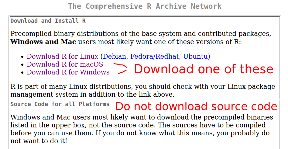
When downloading R from CRAN website, you should see a picture similar to this. Download a version for Windows or Mac, depending on the computer you use.
A good place to download and install R is CRAN website (CRAN stands for Comprenensive R archive Network). You should download the version that corresponds to your operating system, in most OS-s just double-clicking on the icon of the downloaded will invoke the corresponding installer. Accept the default parameters, unless you know better. As of this writing, the most recent R version is 4.3.2.
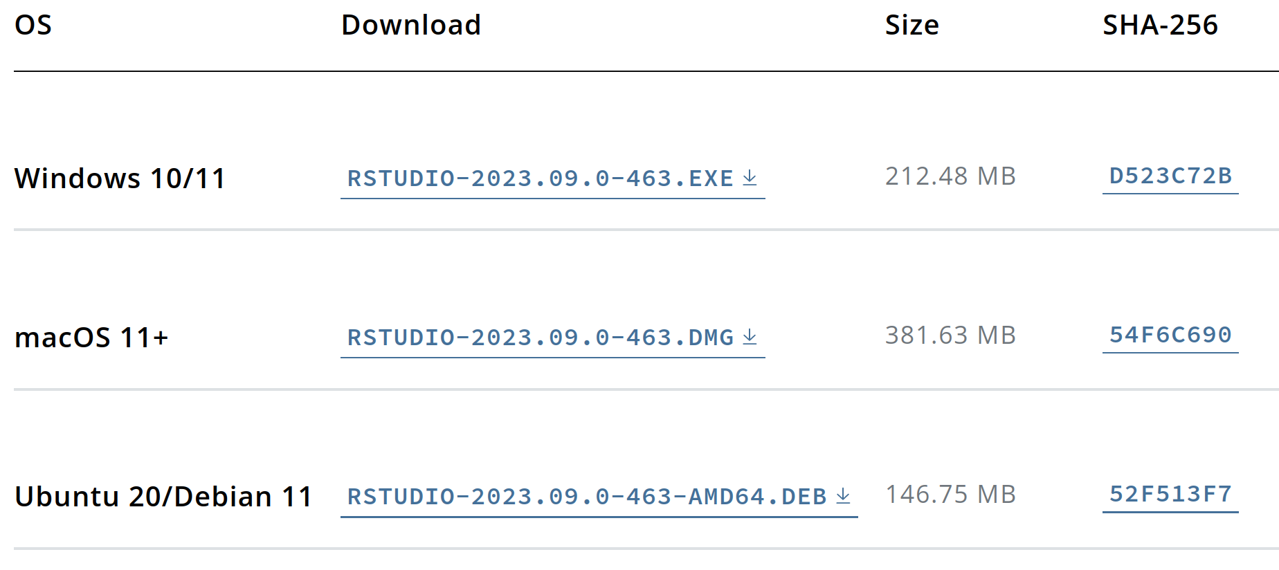
Downloading RStudio. From the list like this, pick the version that corresponds to your computer. Note that the exact version numbers may be different.
RStudio can be downloaded from its download page. Click the one that corresponds to your OS. Again, accept the default values unless you know better. As of this writing, the most recent version of RStudio is 2023.09.0.
Note that you should install R before you install RStudio. This is because RStudio is looking for R during installation, and may complain and get configured in a wrong way if it cannot find it. When you get to the RStudio dowload site, there will be a reminder for this.2.2 First look at RStudio
After you have successfully installed both, the next step is to start Rstudio and take a quick tour of how it can be used. RStudio can be started either by double-clicking on its icon, or though your desktop menus. After fresh start, you should see a picture resembling the one below: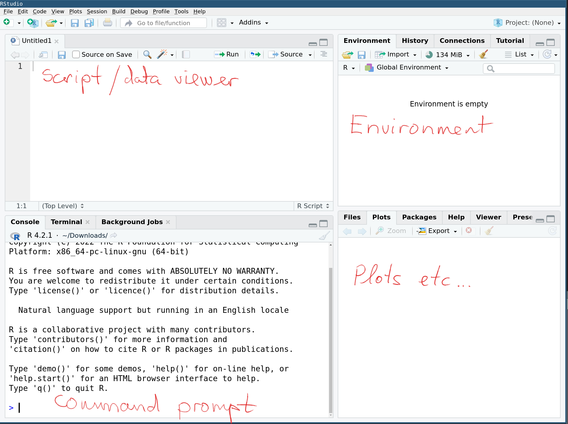
RStudio default layout. After starting it for the first time, you should see something similar. The main window is split into four “panes” that are dedicated to different tasks.
The main window is split into for “panes”. By default, the upper–left pane is dedicated to scripts (code) and the data viewer (See Section 3.7). This pane may be missing if you do not have any scripts open. The upper-right contains information about the working environment or workspace. This contains a list of all dataset and other workspace variables. That pane also contains the command history, and other options. The lower-left pane contains the command prompt (Console). This is one of the central ways to interact with R, more about it below. Finally, the lower–right pane contains a list of plots, files, packages, the help window, and other tasks.
All these panes can be
moved, re-sized or closed. For instance, Ctrl-1 (Cmd-1 on Mac)
makes the script pane active while Ctrl-Shift-1 zooms into the
script window by closing all other panes. Use
Ctrl-Shift-0/Ctrl-Alt-Shift-0 (linux/windows) to
return to the default view. These are extremely helpful keyboard
shortcuts that make working with Rstudio much more effective.
There are many more shortcuts, take a look at the View menu and the
options there.
2.3 Creating projects
A frustrating problem that happens to many beginners is that your software, such as RStudio, cannot easily find the files you want it to find, and you cannot find the files you just created. The best way to overcome this problem when using RStudio is to use projects.
Projects are just separate sets of files and folders that are relevant for different tasks, for instance for all the work you do in this class. You may also want to create separate projects for different problem sets, but that is less important. After you have created a project, you can just click on the corresponding project icon to re-open RStudio in the correct folder with all the right files open.
But before you create a project, you should create a folder where the project will live. As a minimum, I recommend to have a separate folder for this class, but you also may want to have separate ones for some homework assignments. You can use your operating system’s tools, such as Windows File Explorer, or Mac’s Finder. It does not matter much where do you put the folder–as long as you know where it is. You need to be able to locate the folder, and files therein, but from your OS file manager, and from within RStudio!
If in doubt, just make the folder on your desktop. The figure below shows just that–a folder “info180” located at the desktop (on Windows). At left, the same folder opened in the RStudio file pane, and at right, it is opened in the file manager (in File Explorer).
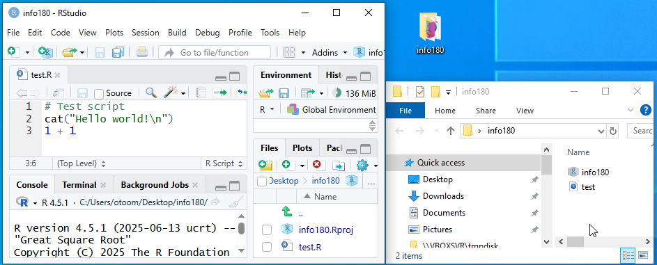
info180 folder on Windows Desktop.
In both views–inside RStudio and the file manager, you can see that
the folder contains two files: the info180 project file (see below),
and a test script file. You can also see that the file manager does
not show the extensions, .Rproj and .R respectively, while RStudio
does. Extensions are very important when loading data using code.
If you later download datasets, imags, or other files that you want to access from R, just move those into the corresponding folder, next to the project and test script.
Creating a project in an existing folder.
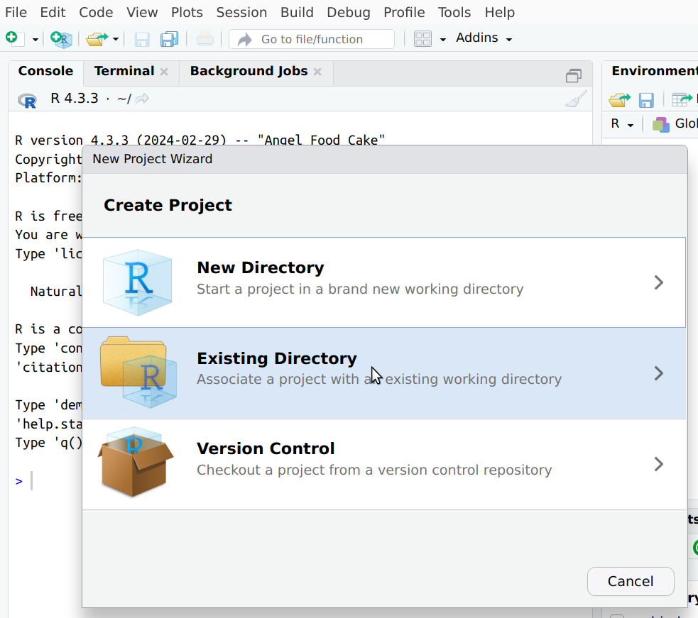
In order to create a project you broadly need to follow these steps:
- Create the folder where you want to keep the files that you need for this project.
- From menu, select File -> New Project. It offers you a few different options (see the figure).
- Pick Existing Directory if you already created the folder,
otherwise and browse to the one you just created. If not, you can
create it here with New Directory.
- Finally, click Choose and Create Project.
RStudio restarts, and now you are working within the project.
Rstudio with a demo project open (upper window) and Rstudio project icon in the folder (in the lower window).
In the example image here, we see a project that contains just one file–hello.R. This is opened in RStudio above. Below, you see the project folder (called info201) that contains the same file, and the blue RStudio project icon (highlighted).
Next time when you want to work on the same project, you just double-click on the project icon in the correct folder. This will ensure that you have only those files and folders open that are relevant for this project.
2.4 Working with R in Rstudio
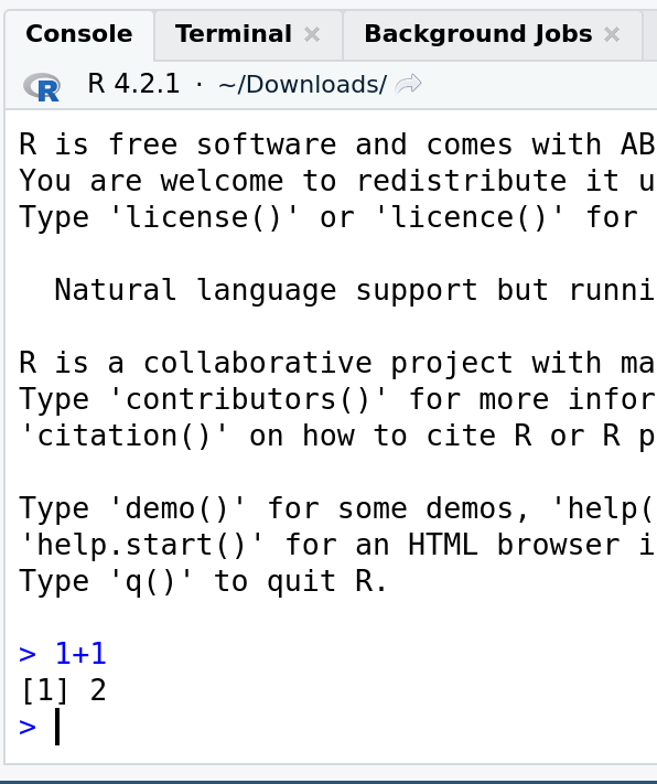
Issuing a simple command at the command prompt. We write “1+1” at the
prompt, followed by Enter. R replies by “2”.
The simplest way to interact with R is through the command prompt.
One can use this as a simple calculator (you can also use it as a very
advanced calculator but that is not what we care about right now
😂). For instance,
let’s compute “1 + 1”. This can be achieved by writing “1 + 1” at the
prompt, followed by Enter. R replies by “2”.1
Further below, we demonstrate the commands using light-gray blocks, the example above will look like
## [1] 2Issuing commands directly on the command prompt is useful for simple tasks like quick calculations or a very simple data analysis. For more complex tasks we want to use scripts (see Section 2.7).
2.5 Workspace variables: remembering your results
Sometimes we do not want just to compute a number but we also want to re-use it later. Hence we have to store it in memory. This can be done by giving it a name. Instead of just computing “1 + 1” and printing the result, we can give the result a name (e.g. “sum”) like this:
Here is the anatomy of the command:
- The right hand side of it,
1 + 1is the same as above (it is called expression). R computes the answer (and gets “2”). sumis the name that we can use to refer to the number later. It is called variable name.- the small arrow,
<-tells R to store the computed result under that name. It is called assignment operator.
You can imagine that variables are boxes in your computer memory. These boxes can contain various things, numbers (as here), text, or the whole datasets. Each box has a label (variable name). So we have just made a box labeled “sum” that contains number “2”. And later we can use the labels instead of the box content. This is somewhat similar like writing a mathematical formula. For instance, we can write surface area of a circle as \[\begin{equation} S = \pi \cdot r^2. \end{equation}\] This is always correct, no matter what is the exact value of radius \(r\).
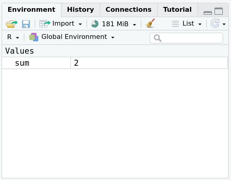
Workspace pane after creating a variable sum that equals “2”
But note what happens in the Environment pane top-right: the previous empty pane will have a list of “Values”, currently consisting of a single value called “sum” that equals to “2”.
However, the answer was not automatically printed on the console, unlike before when we did not store the result. Now it “went to the box”, instead of going printed to the console. If you want to print it explicitly, you can do it by just writing the name at the command prompt:
## [1] 2Later we also encounter a different type of variables, ones that are stored in datasets, not in the workspace. So when we need to be more precise, then we call the variables in your workspace (“environment” pane) either environment variables2, or workspace variables (because the Global Environment is also called workspace). The variables we later encounter in datasets we call data variables. But in unambiguous situations we call both just “variables”.
You cannot label variables just as you wish–there are certain rules.
It should start
with a letter, and can contain letters, numbers, and a few other
symbols. So sum, sum1, S1 are valid variable names, but 1s is
not.
Be also aware that the names are case sensitive, so sum and
Sum are different things.
Exercise 2.1 Try out a few valid and invalid variable names. You can try something like
and
Try out the following:- variable name that begins with a number (like
1x) - variable name that contains space (like
x 1) - variable name that contains a dot (
x.1) - variable name that contains underscore (
x_1) - variable name that contains a dollar sign (
x$1)
What happens? What are the exact error messages?
See the solution
2.6 Data types
So far, we only worked with numbers. But R also has two other very important data types, character string and logical (Boolean). Here we discuss the data types a little more.
2.6.1 Numeric
The easiest data type to understand are numbers, numeric in R parlance. These are just plain numbers that support common mathematical operations, such as+,-,*,/: addition, subtraction, multiplication, division^: exponentiation%/%: integer division: for instance,5 %/% 2is two, because integer division ignores all fractions.%%: modulo (reminder),5 %% 2is one, because the remainder of five divided by two is one.
The order of operations is the same as in ordinary mathematics–exponentiation is done first, thereafter multiplication and division, and finally addition and subtraction. If you are unhappy with the order, you can always use parenthesis to do it differently:
## [1] 7## [1] 9Numbers are sometimes printed using scientific notation like
## [1] 6.750007e-06## [1] 3.937376e+15The “e” in the results should be understood and “ten-to-power-of”, so 6.750007e-06 is \(6.750007\cdot 10^{-6}\) and 3.937376e+15 is \(3.937376\cdot 10^{15}\).
TBD: data types character, logical
2.7 Writing scripts: repeating and improving your commands
Issuing commands at the command prompt is useful for simple tasks. But for more complex tasks, it is advisable to write all your commands underneath each other in the script window, and execute all those together. The main advantage of this approach is that you can easily edit and change your commands if you change your mind, or if you spotted problems in your previous commands.
Here is a small example. Let’s compute the area of a circle with radius 2 (the formula is \(\pi \cdot r^2\)). We can compute it directly:
## [1] 12.56Note that the asterisk * is used for multiplication, and caret ^
for exponentiation.
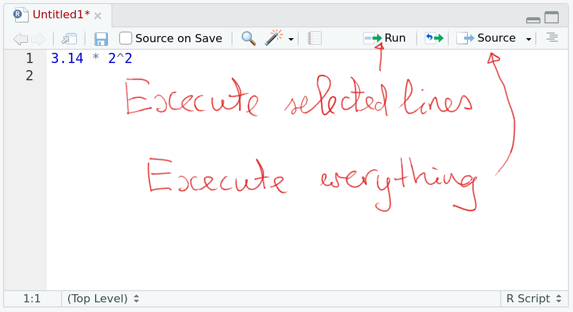
Writing the command in the script window. “Run” for executing the highlighted lines and “Source” for executing everything are highlighted.
Instead of writing this directly in the command prompt, we can write it into the script window (the top-left pane) instead. It is basically just a text editor where you can write your commands, but unless you tell computer to execute those (called running, sourcing or just executing), those are just sitting there and doing nothing. RStudio offers two easy ways to execute the commands: “Run” and “Source”. “Run” only runs the commands you have highlighted. This is handy if you have many commands in the window, and you only want to execute a few. “Source”, in contrary, executes everything in that window. This is good if you have written multiple commands to achieve a final goal, and you want to do all that in one go.
Why do you may want to use scripts instead of just issuing commands? There are a few reasons:
- Scripts are easy to edit. If you made a mistake when you first wrote down the commands, or maybe changed your mind about how you want to proceed, then you can just fix and change the relevant lines and re-run it again. No need to re-write all the commands.
- In a similar fashion, scripts are very handy if you develop your ideas. You can start simple, see how it works, and correct the old ones and add more commands as you gain understanding of your problem.
- A different reason is that the scripts are excellent documents. As the computer commands are precise, they tell exactly what did you do. If you are unsure how exactly did you compute a particular result, it is just to look at the commands stored in the script.
Writing scripts is called scripting, and it is the same thing as programming. In this course we stay with very basic scripting and leave more advanced tools for dedicated programming courses.
What happens when we run the whole script using the Source button?
At the first attempt nothing
interesting. We can see message like
source("~/.active-rstudio-document") appearing at the command
prompt. But we do not see any answer. The problem here is that
unlike with commands that are issued directly at the prompt, the
results executed in scripts are not automatically printed. But we can
amend the script to include printing. Editing the commands is exactly
what the scripts are made for.
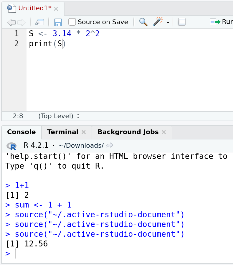
The previous script amended for printing. Now the result, 12.56, is visible at the command prompt.
We do the following: first we save the result under name S (for
“surface”), and then we explicitly print it using print(S). When
hitting the Source button now, the result, 12.56, pops up in the
command window.
But note that now the Environment pane includes two names: “sum” from earlier, and now also “S”, the same 12.56 we calculated here.
Note also that when using Run instead of Source, the results are printed automatically, so no need to add explicit printing if you use that button.
2.8 Packages: re-using work done by others
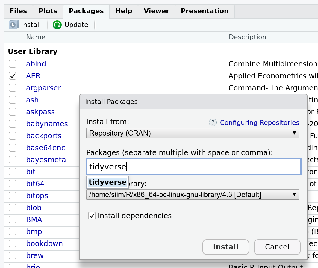
Loading and installing R packages. You can just click the checkbox to load the library, for installing packages you can click the “install” button, and enter the library names to the dialog window.
R has many-many built-in commands. But even more are available in packages. These are external libraries that are not automatically loaded when you start R. In many cases you even need first to download and installed them before you can use those. There are several ways to install packages, the simples one is to use the “Install” button in the Packages tab in the bottom-right pane.
Later, when doing the data analysis, we rely heavily on the tidyverse package. More precisely, tidyverse is a set of packages, not just a single one, but that does not concern us here. We can install tidyverse by hitting the “Install” button and writing “tidyverse” in the package name bar. The other options can normally be left as they are. Depending on your operating system and the exact package versions available, the installation process may ask if you want to install the binary or source packages. We recommend to install the binary versions3–unless you know better what to do. As tidyverse is a large package, the installation process can take a few minutes.
Exercise 2.2 Alternatively, packages can be installed using the command
install.packages. Install lubridate, a package that provides a
set of very useful date and time–related functions by issuing command
at the command prompt.
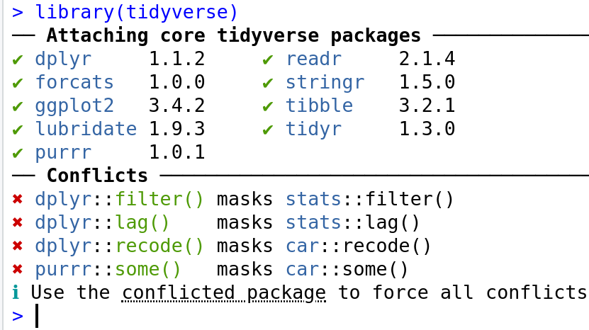
Loading tidyverse. R gives a number of messages, including conflict reports. Here they describe similar command both in tidyverse and other packages that can potentially lead to wrong results.
After installation, the packages are downloaded and ready to be used.
But they are still not available at the command prompt (nor in
scripts). To make these available, you need to issue command
library. For instance, let’s make tidyverse functionality
available:
R responds with a number of messages that we do not have to be concerned here. Alternatively, you can check the box next to the library name at the “Packages” pane (see the image above).
Now we can use some of the tidyverse functionality. One of the most
useful tools is the “pipe operator” %>%. This allows certain commands to
be executed in the logical order, almost like reading from a cooking
recipe. For instance, we can give the command
## [1] 1.414214to compute square root of two. If your tidyverse is installed and
loaded, then R replies 1.414214. If something went wrong, you get
an error message.
The “piped” approach can be understood as “take number two, and compute square root of it”. While here it may feel weird, it turns out to be an extremely useful way of analyzing data later, see Section (pipelines).
Exercise 2.3 Put the same commands in the script window. But
this time split the sqrt function to the next line:
Run these lines using the Run button. Do you get the same result?
See the solution
Exercise 2.4 Now restart RStudio without laoding tidyverse. You can just exit it and re-start it, but do not load tidiverse!
Re-run the command 2 %>% sqrt(). What happens?
See the solution
2.9 Getting help
An extremely important task in data processing is to learn more. No one can ever learn and remember all the commands and functions of sofware and even professionals who are fluent in the basic tools, frequently need to consult various help materials for more specific tasks.
2.9.1 Available help sources
First, the most obvious source are the other sections of these notes. In particular, R Cheatsheet contains a quick overview of basic commands and a reference to the relevant pages.
R has also a built-in help system that one can access as
?commandto read the built-in help for that command, or??topicto find all kinds of help files related to that topic. RStudio also has a dedicated help window with search bar in the bottom-right pane.
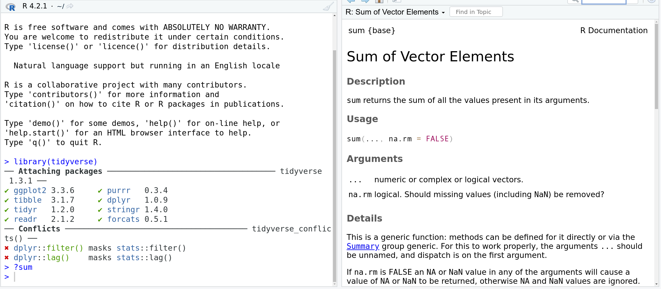
Help window in RStudio. Note the ?sum as the last command at the
command prompt at left. The right-hand window displays the built-in
help for the “sum” command.
- The third reading source I can warmly recommend is R for Data Science by Hadley Wickham and Garrett Grolemund. It is a very good introduction to data processing and how to do it with R. However, it is oriented to a more technical reader.
Unfortunately, for beginners, it is not easy to use the existing
sources for help. For instance, the ?command help assumes you have
at least a vague idea what kind of commands to use. Also, the help
files are written with a much more tech-savy user in mind so even if
you find the correct page, you may miss some of the crucial
information there.
A second problem is that computer help texts are typically oriented to questions like “how can I achieve X on computer”, where “X” is typically a very specific task. For instance, you may easily find information about how to rename columns in a data frame. But that assumes that you are able to design a data processing pipeline in your mind where you find that renaming variables might be a good thing to do. If your problem is that you do not really know what the “X” might be, then you cannot ask such questions, and cannot easily use related answers.
So there is no way around learning, thinking about how to process data, and playing with examples. In these notes we give various examples of data processing that will help you to develop such skills and be able to read the existing documentation.
2.9.2 Asking for help
Finally, we should also talk about how to ask for help. There is nothing wrong with asking for help–even professionals do if often. There is waaay more things to learn than anyone can learn. So everyone asks for help. But it can be asked in a better or in a worse way.
A good way to ask for technical help will be along these lines:
- Tell what do you want to achieve. Not what you do but what do you want to do. This is primarily because understanding the goals helps to understand the question. It may also happen that you are using an unsuitable approach right now, and if experienced people understand what you want to do, then they can give you better suggestions.
- Tell what do you do. Even if you do not “do” anything, you should list here your thoughts related to what kind of steps you consider taking. This helps others to know “where you are”. In order to help you, the other person must be on the same page as you, and this is essentially the description of “the page”.
- Tell what happens when you do this. It is simple to show if you run computer code, but even if you are trying to design a processing pipeline, you can tell something like: I can load data, and can convert the variables I need, but now I am not sure how I should compute the averages…
- Tell what is wrong with your current approach. Sometimes it is easy to see, e.g. you get an error. But this is not always the case. What is wrong with your plot? Others may think it is a perfectly fine plot, unless you tell them that it should use different scales, colors or variables.
All these suggestions are more demanding for beginners who do not possess the professional way of thinking and professional vocabulary. This may turn off some of the potential helpers as, essentially, you speak a different language. But others are able to understand what you mean if you explain it clear enough. It may help to be very explicit that you are the beginner by telling something like “this is my first time to load a dataset…”.
More specifically, it replies by
[1] 2. The “[1]” means that this is the first part of the answer, there may be many parts, but we do not need that for now. Just be aware that you tend to see all answers preceded by “[1]”.↩︎Here, “environment variables” is actually a bad name. This is because on computer there is another sort of variables, unrelated to R, that is called “environment variables”. Everyone who is familiar with operating systems will believe you are talking about those instead.↩︎
R will ask if you want to install source versions as those are newer. You should answer “no” at the command prompt.↩︎