Key LPL model parameters In the LPL model (Curtis 1986), four key parameters determine the survival response of cells exposed to ionizing radiation. The four parameters are: - Initial DSB yield Gy-1 cell-1. Specify using the DSB={value} keyword.
- Initial yield of unrepairable (and thus fatal) lesions Gy-1 cell-1. Specify using the FL={value} keyword.
- 1st order DSB rejoining rate. Specify using the LAM={value} keyword or RHT={value} keyword. The LAM and RHT parameters are related by LAM = LN(2)/RHT.
- Rate of pairwise damage interaction (2nd order DSB rejoining rate). Specify using the ETA={value} keyword.
In addition to these four key radiosensitivity parameters, several other parameters can be adjusted to better reflect the biological properties of a particular type of cell, such as the DNA, NC, A0 (or B0), and GAM parameters. Refer to the Biophysical Parameters section of the manual for a complete list biological parameters and their definitions.
Tip: The widely used LQ survival formula, S = exp{-D(a + bGD)}, is a low dose and dose rate approximation for the LPL model. Here, D is the absorbed dose, G is the dose protraction factor that accounts for dose-rate and dose-fractionation effects, and a and b characterize intrinsic radiosensitivity. Estimates of LQ radiosensitivity parameters (a and b) derived from the LPL radiosensitivity parameters are reported in the VC output file.
Exercise 1 - Paste the contents of LPL sample file #1 into a new ASCII input file called lpl1.inp (see Getting Started on the Tutorial for help with this step).
- Modify lpl1.inp to generate several single-dose exposure scenarios. Setup scenarios to delivery absorbed doses from 0 to 10 G and deliver the doses at 1,000 Gy/hour).
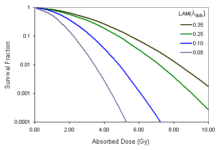
- Generate survival curves for repair half-times (RHT parameter) of 0.25 h, 0.5 h, 1 h, 2 h, 4 h. Plot surviving fraction (y-axis, log scale) vs. absorbed dose (x-axis, linear scale). The plot should look similar to Figure 1.
Questions- Does the surviving fraction tend to increase, decrease or stay the same as the repair half-time increases?
- Does the LQ radiosensitivity parameter a change as the repair half-time changes (see VC output file for value of a)? If so, does a increase or decrease as the repair half-time increases?
- Does a/b ratio change as the repair half-time changes? If so, does a/b increase or decrease as the repair half-time increases?
Increase the DSB yield by a factor of two (DSB parameter). Does a increase, decrease or stay the same? Does a/b increase, decrease or stay the same? Identify a formula to relate changes in a and a/b to changes in the initial DSB yield. Figure 1. Effects of the DSB rejoining rate parameter LAM on cell survival. Figure 1. Effects of the DSB rejoining rate parameter LAM on cell survival.
Exercise 2- Create a copy of the lpl1.inp file (Exercise 1); rename the file to lpl2.inp.
- Change the dose rate from 1,000 Gy/hour to 0.01 Gy/hour.
- Set the half-time for DSB rejoining to 4 h. Plot surviving fraction (y-axis, log scale) vs. absorbed dose (x-axis, linear scale).
Questions - Re-run the simulation with repair half-times of 0.1 h, 0.5 h, and 2 h. Is the survival response of this cell sensitive to the value of RHT (and hence LAM) under low dose rate exposure conditions?
- Set the repair half-time to 2 h and then re-run the simulation with values of ETA equal to 10-5 h-1 and 10-
3 h-1. Is the survival response of this cell sensitive to the value of ETA under low dose rate exposure conditions?Increase the initial yield of fatal lesions by a factor of 2 (FL parameter). Is the survival response of this cells sensitive to the value of the FL parameter?Determine a formula to estimate FL from the surviving fraction S for low dose rate exposure conditions. Hint: The LQ protraction factor, G, approaches zero for very low dose rates so that S ~ exp{-aD}. Solve for a (which is related to the FL parameter). Will estimates of FL be too high or too low if a survival fraction for an acute exposure (high dose rate) is used instead of survival data for a low dose rate exposure conditions?
Exercise 3- Create a copy of the lpl1.inp file (Exercise 1); rename the file lpl3.inp.
- Set the dose rate to 25 Gy/h.
- Set the repair half-time equal to 0.25 h (RHT=0.25). Then set ETA = LN(2)/(RHT*1000). Plot surviving fraction (y-axis, log scale) vs. absorbed dose (x-axis, linear scale).
- Repeat step 3 for repair half-times of 0.75 h, 2 h, and 4 h, i.e., compute ETA for each repair half-time using the formula ETA = LN(2)/(RHT*1000), run the simulation and then add the survival curve to the plot. Upon completing step 4, the plot should have four curves (one for each combination of RHT, ETA).
Questions- Compute the ratio of LAM/ETA for each of the repair half-times (compare to value reported in VC output file). Does this ratio increase, decrease or stay the same as the repair half-time increases (this is not meant to be a trick question; the answer is readily apparent if you think about the method used to compute ETA from the RHT)?
- Does the value of a increase, decrease or stay the same as the repair half-time increases?
- Does the value of a/b increase, decrease or stay the same as the repair half-time increases?
- Are changes in a and a/b proportional to the repair half-time or the ratio LAM/ETA?
|


 Figure 1. Effects of the DSB rejoining rate parameter LAM on cell survival.